In [1]:

%matplotlib inline

============================ Underfitting vs. Overfitting ============================

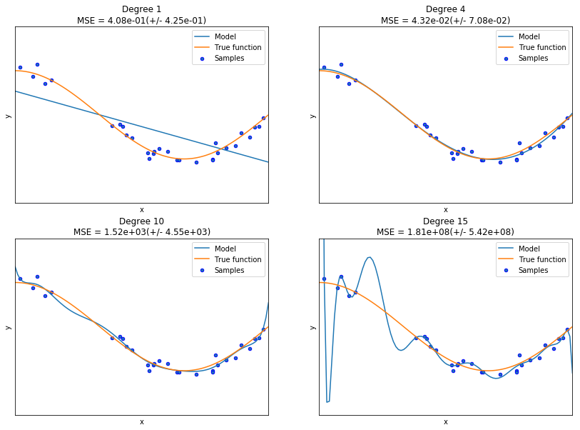
This example shows how underfitting and overfitting arise when using polynomial regression to approximate a nonlinear function, \(y =1.5 \cos (\pi x).\)

The plots shows the function \(y(x)\) and the estimated curves of of different degrees.

We observe the following:

• The linear function (polynomial with degree 1) is not sufficient to fit the training samples—this is underfitting.
• A polynomial of degree 4 approximates the true function almost perfectly and gives the smallest MSE.
• For higher degrees, the model overfits the training data, and the mean-squared errors (MSE) become very large–the model is learning the noise in the training data.

We evaluate quantitatively overfitting / underfitting by using cross-validation and then calculating the mean squared error (MSE) on the validation set. The higher the value, the less likely the model generalizes correctly from the training data since it is brittle.

In [2]:

import numpy as np
import matplotlib.pyplot as plt
from sklearn.pipeline import Pipeline
from sklearn.preprocessing import PolynomialFeatures
from sklearn.linear_model import LinearRegression
from sklearn.model_selection import cross_val_score

def true_fun(X):
    return np.cos(1.5 * np.pi * X)

np.random.seed(0)

n_samples = 30
degrees = [1, 4, 10, 15]

X = np.sort(np.random.rand(n_samples))
y = true_fun(X) + np.random.randn(n_samples) * 0.1

plt.figure(figsize=(14, 10))
for i in range(len(degrees)):
    ax = plt.subplot(2, 2, i + 1) 
    plt.setp(ax, xticks=(), yticks=())
    polynomial_features = PolynomialFeatures(degree=degrees[i],                                            include_bias=False)
    linear_regression = LinearRegression()
    pipeline = Pipeline([("polynomial_features", polynomial_features),
                         ("linear_regression", linear_regression)])
    pipeline.fit(X[:, np.newaxis], y)

    # Evaluate the models using cross-validation
    scores = cross_val_score(pipeline, X[:, np.newaxis], y,
                             scoring="neg_mean_squared_error", cv=10)

    X_test = np.linspace(0, 1, 100)
    plt.plot(X_test, pipeline.predict(X_test[:, np.newaxis]), label="Model")
    plt.plot(X_test, true_fun(X_test), label="True function")
    plt.scatter(X, y, edgecolor='b', s=20, label="Samples")
    plt.xlabel("x")
    plt.ylabel("y")
    plt.xlim((0, 1))
    plt.ylim((-2, 2))
    plt.legend(loc="best")
    plt.title("Degree {}\nMSE = {:.2e}(+/- {:.2e})".format(
        degrees[i], -scores.mean(), scores.std()))
plt.show()