Subsurface-Offset Image Volumes

Extended Imaging, Velocity Analysis, and the Road to FWI

Felix J. Herrmann

Schools of EAS, CSE, ECE — Georgia Institute of Technology

2026-04-01

Subsurface Image Volumes and Migration Velocity Analyses

Felix J. Herrmann

School of Earth and Ocean Sciences — Georgia Institute of Technology

Based on Hou and Symes (2015), Hou and Symes (2016), and Hou and Symes (2018).

Outline

Motivation — Why extend the image?
Born modeling recap — Connection to RTM and LSM lectures
The Born inverse problem — Overdetermination and velocity dependence
Extended Born modeling — Subsurface-offset extension
Extended imaging operators — RTM vs. approximate inverse
Preconditioning — Left and right weight operators
Extended least-squares migration — Fitting data with any velocity
Weighted conjugate gradient — Accelerating convergence
DSO velocity analysis — Focusing as a velocity criterion
Numerical examples — Marmousi and field data
Limitations of WEMVA — Artifacts and the road to FWI

William W. Symes

Noah Harding Professor Emeritus
Computational & Applied Mathematics, Rice University

Founded The Rice Inversion Project (TRIP) — 25+ years of industry-sponsored research
Pioneered differential semblance optimization for migration velocity analysis
SIAM Fellow; Desiderius Erasmus Prize (EAGE, 2015); Ralph E. Kleinman Prize (SIAM)
Key insight: use the approximate inverse (not the adjoint) for velocity analysis

Motivation

Dual Purpose of Subsurface-Offset Image Gathers

Subsurface-offset common-image gathers (CIGs) serve two purposes:

Migration-velocity analysis: Focusing of CIGs or flatness of common-angle gathers indicates the velocity model is correct
Directional scattering information: When the velocity model is correct, CIGs contain amplitude-versus-angle (AVA/AVP) information

This lecture

We focus on velocity model building — using the extended image volume to update the background velocity $v_0$. The directional/AVA aspect will be covered later.

Recall: The Two-Parameter Inverse Problem

From our RTM and LSM lectures, we know:

RTM computes the gradient of the FWI objective — it is the adjoint $\mathbf{F}^T$, not the inverse
LSM solves $\mathbf{F}^T\mathbf{F}\,\delta\mathbf{m} = \mathbf{F}^T\mathbf{d}$ to deconvolve illumination effects
Both require a kinematically correct background velocity $v_0$

Key question

What if $v_0$ is wrong? Can we still extract useful information from the image to update the velocity?

Born Modeling Recap

Connection to Previous Lectures

Born Approximation — Continuous Form

The velocity is decomposed as $v(\mathbf{x}) = v_0(\mathbf{x}) + \delta v(\mathbf{x})$, where $v_0$ is smooth and $\delta v$ contains reflectors (Hou and Symes 2015).

The Born modeling operator $F[v_0]$ maps reflectivity $\delta v$ to scattered data:

\[ (F[v_0]\delta v)(\mathbf{x}_s, \mathbf{x}_r, t) = \frac{\partial^2}{\partial t^2} \int d\mathbf{x}\, d\tau\, G(\mathbf{x}_s, \mathbf{x}, \tau) \frac{2\delta v(\mathbf{x})}{v_0(\mathbf{x})^3} G(\mathbf{x}, \mathbf{x}_r, t - \tau) \tag{1}\]

This is Equation 6 of Hou and Symes (2018). Compare with discrete expression

\[ \begin{align}\mathbf{J}&=\nabla\mathcal{F}[\mathbf{x}_0]\\ &=-\mathbf{P}_r\mathbf{A}^{-1}[\mathbf{x}]\mathrm{diag}\big(\frac{\partial\mathbf{A}[\mathbf{x}]}{\partial\mathbf{x}}\mathbf{A}^{-1}[\mathbf{x}]\mathbf{P}^\top_s\mathbf{q}\big)\Bigr|_{\mathbf{x}_0} \end{align} \]

Connection to Lecture Notation (RTM)

In the discrete notation of our RTM lecture:

Continuous (Papers)	Discrete (Lecture A)
$F[v_0]\,\delta v = \delta d$	$\mathbf{F}\,\delta\mathbf{m} = \delta\mathbf{d}$
$G(\mathbf{x}_s, \mathbf{x}, t)$	$\mathbf{A}^{-1}(\mathbf{m})\,\mathbf{q}_s$
$F^*[v_0]\,\delta d$ (RTM)	$\mathbf{F}^T\,\delta\mathbf{d}$ (adjoint)
Imaging condition	$[\nabla_\mathbf{m} J]_i = \sum_s \sum_k v_s(x_i,t_k)\,\ddot{u}_s(x_i,t_k)\,\Delta t$

Note

The Born modeling operator $F[v_0]$ in the papers corresponds to the stacked Jacobians $\mathbf{F} = [\mathbf{J}_1^T, \ldots, \mathbf{J}_{n_s}^T]^T$ from our LSM lecture $.

The Born Inverse Problem

The Born inverse problem seeks $v_0$ and $\delta v$ such that $F[v_0]\,\delta v \approx d$ (Hou and Symes 2018).

This corresponds to the LS-RTM problem we discussed before in class
Data fit is impossible unless $v_0$ is kinematically correct to within a half-period error in traveltime prediction (Symes 2008)
This is because we are solving an overdetermined problem: the data dimension exceeds the model dimension (e.g., 5D data vs. 3D model)
Data fit is only possible in the special case of correct velocity

The way out

If $\delta v$ is extended to depend on an extra dimension (subsurface offset $h$), i.e., replaced by $\delta\bar{v}(\mathbf{x}, h)$, then any model-consistent data can be fit with essentially any $v_0$ by proper choice of $\delta\bar{v}$.

Extended Born Modeling

Subsurface-Offset Extension

Subsurface Offset — The Idea

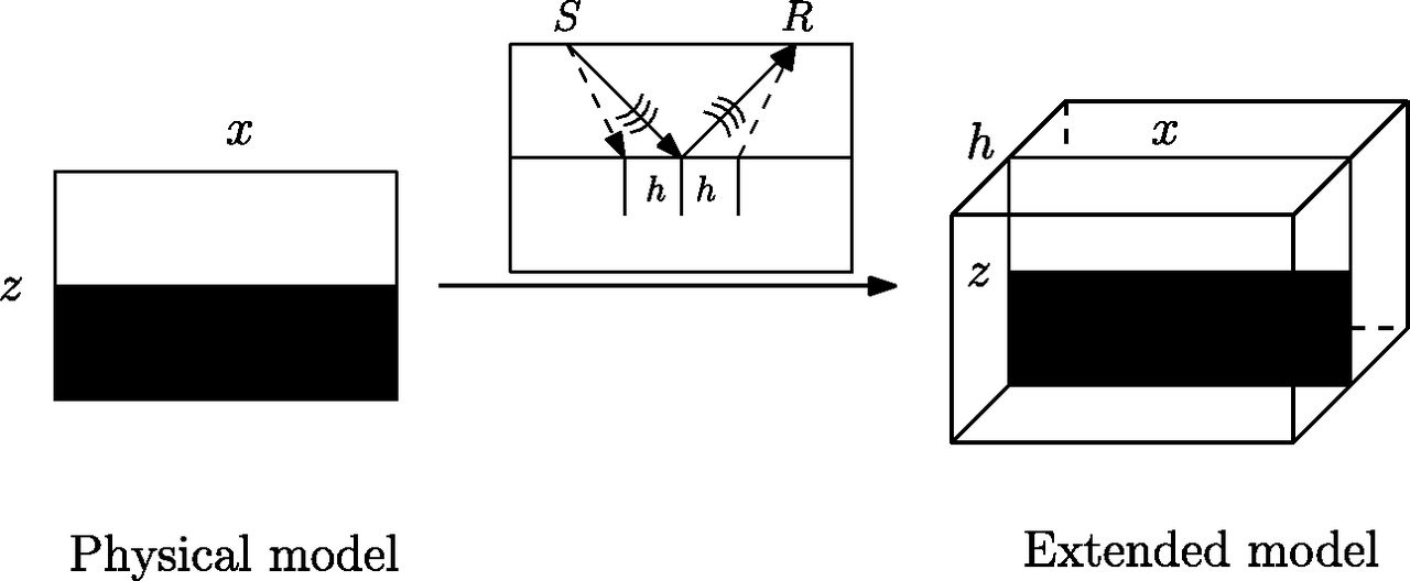
Sketch of the subsurface offset extension. The subsurface offset $h$ is half the distance between subsurface scattering points. This extension allows stress to produce strain at a distance (Hou and Symes 2016).

Extended Born Modeling Operator

The reflectivity $\delta v(\mathbf{x})$ is replaced by $\delta\bar{v}(\mathbf{x}, h)$, and the extended Born modeling operator $\bar{F}[v_0]$ is defined as (Hou and Symes 2018, Eq. 7):

\[ (\bar{F}[v_0]\delta\bar{v})(\mathbf{x}_s, \mathbf{x}_r, t) = \frac{\partial^2}{\partial t^2} \int d\mathbf{x}\, dh\, d\tau\, G(\mathbf{x}_s, \mathbf{x} - h, \tau) \frac{2\delta\bar{v}(\mathbf{x}, h)}{v_0(\mathbf{x})^3} G(\mathbf{x} + h, \mathbf{x}_r, t - \tau) \tag{2}\]

Here $h$ is half the distance between sunken source and sunken receiver in Claerbout’s survey-sinking imaging condition (Claerbout 1985).

Physical meaning: We now allow reflection at a distance — a nonphysical extension that matches the model dimension with the data dimension.

Extended Imaging Operator (RTM)

The extended imaging operator is the adjoint of $\bar{F}$ — i.e., extended RTM (Hou and Symes 2018, Eq. 8):

\[ I(\mathbf{x}, h) = (\bar{F}^*[v_0]\,d)(\mathbf{x}, h) = \frac{2}{v_0(\mathbf{x})^3} \int d\mathbf{x}_s\, d\mathbf{x}_r\, dt\, d\tau\, G(\mathbf{x}_s, \mathbf{x} - h, \tau)\, G(\mathbf{x} + h, \mathbf{x}_r, t - \tau) \frac{\partial^2}{\partial t^2} d(\mathbf{x}_s, \mathbf{x}_r, t) \tag{3}\]

In our lecture notation, the extended RTM corresponds to:

\[\boldsymbol{\delta}\bar{\mathbf{v}}[\mathbf{x}, h_x]=\bar{\mathbf{F}}^T\,\delta\mathbf{d}=\sum_s\sum_t\mathbf{v}_s[\mathbf{x}+h_x]\ddot{\mathbf{u}}_s[\mathbf{x}-h_x,t]\]

where $\bar{\mathbf{F}}$ now depends on both spatial position $\mathbf{x}$ and subsurface offset $h$. Corresponds to the cross-covariance between the forward and adjoint wavefields.

Reflection Data

We define the reflection data as the difference between nonlinear data and data simulated in the background-velocity model (Hou and Symes 2018, Eq. 3):

\[ \delta d = \mathcal{F}[v] - \mathcal{F}[v_0] \approx F[v_0]\,\delta v \]

where $\mathcal{F}[v]$ is the nonlinear forward modeling operator mapping velocity to data.

What Focusing Tells Us

The RTM offset gather with (a) 10% slower velocity, (b) correct velocity, (c) 10% faster velocity; approximate inverse offset gather with (d) 10% slower velocity, (e) correct velocity, (f) 10% faster velocity. All inverted gathers plotted on the same scale (Hou and Symes 2018).

Tip

Energy focuses at $h = 0$ with correct velocity and spreads to nonzero $h$ when velocity is incorrect.

Approximate Inverse Operator

From Adjoint to Inversion

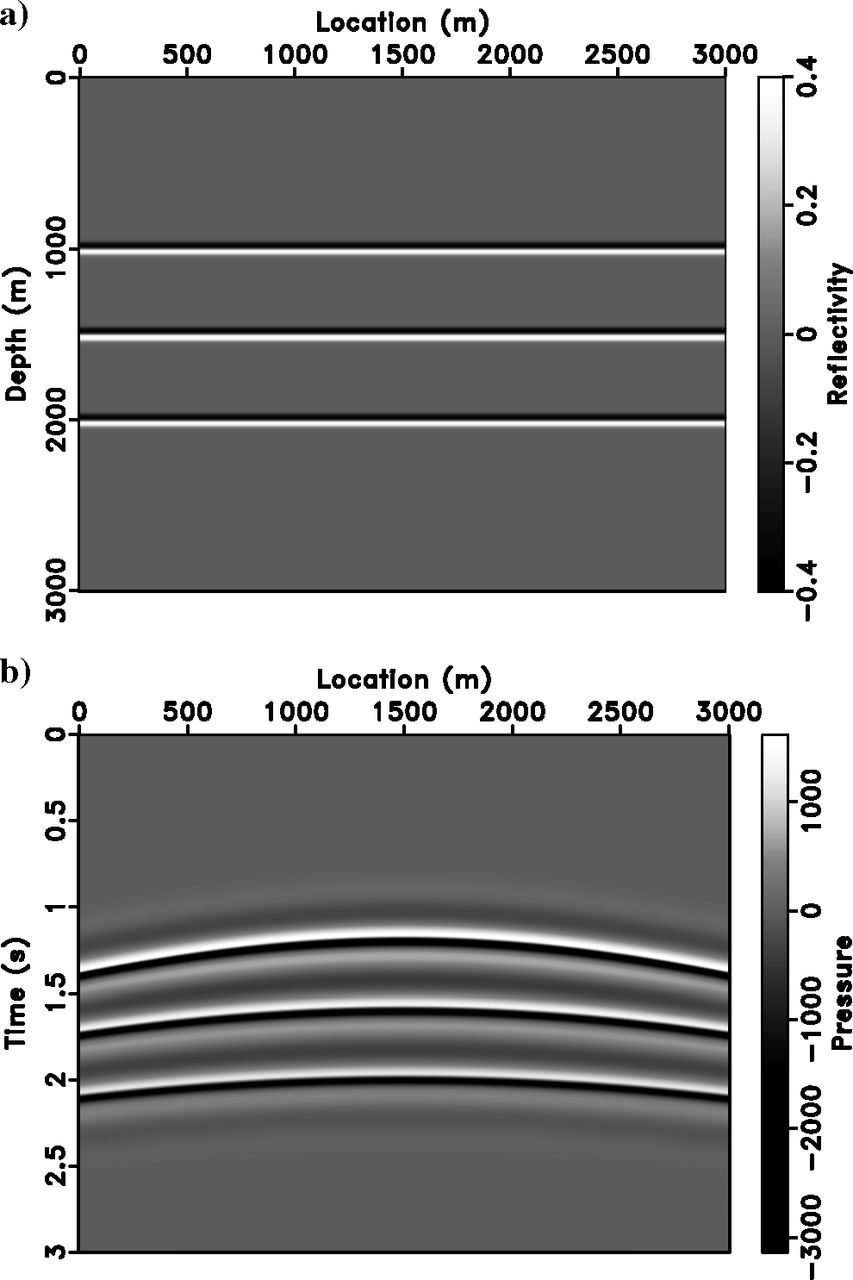
Paper A: Simple Model Setup

Reflectivity model ($\delta v$) with constant background ($v_0 = 2500$ m/s) and one-shot simulated Born data (Hou and Symes 2015).

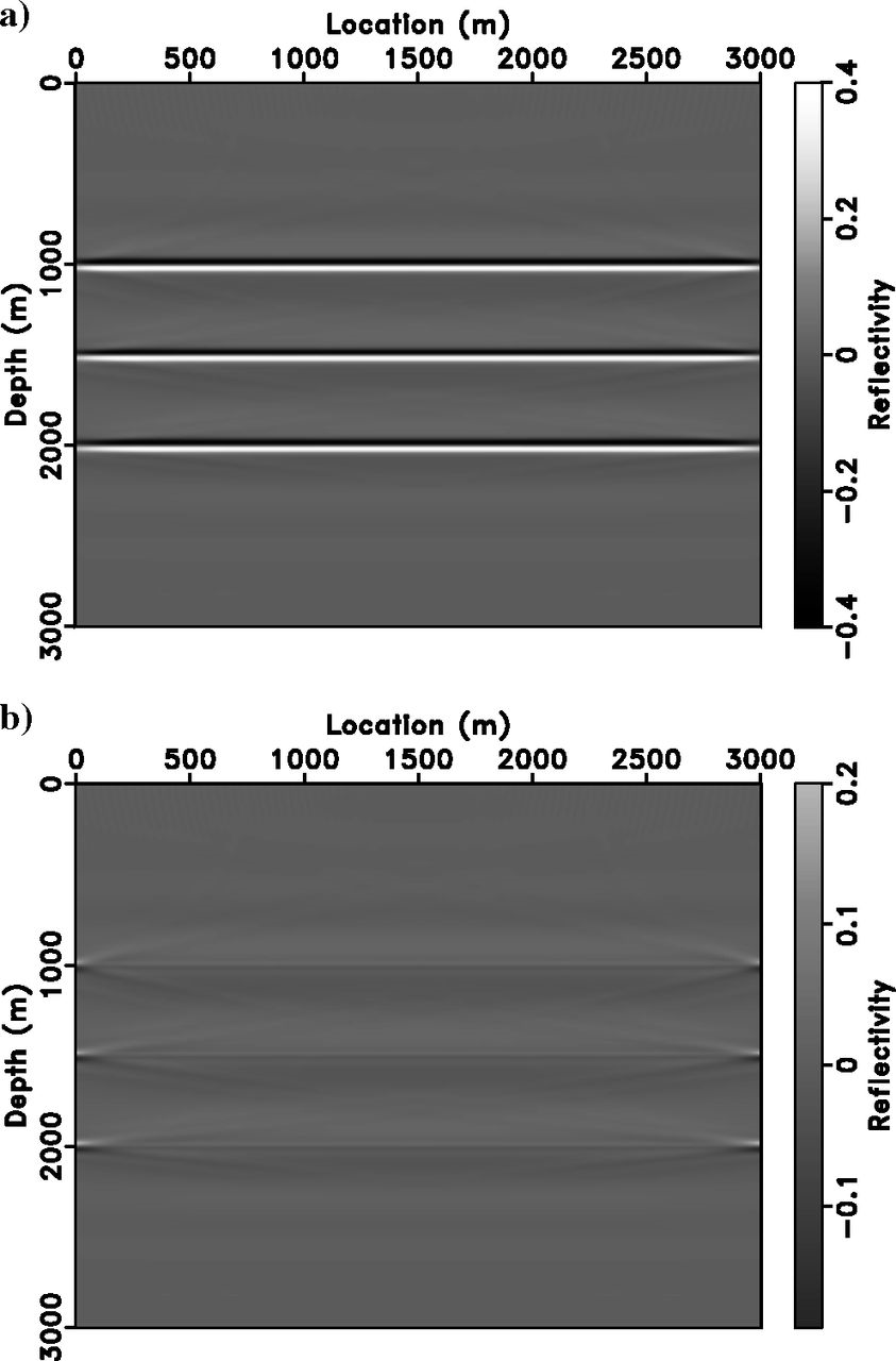
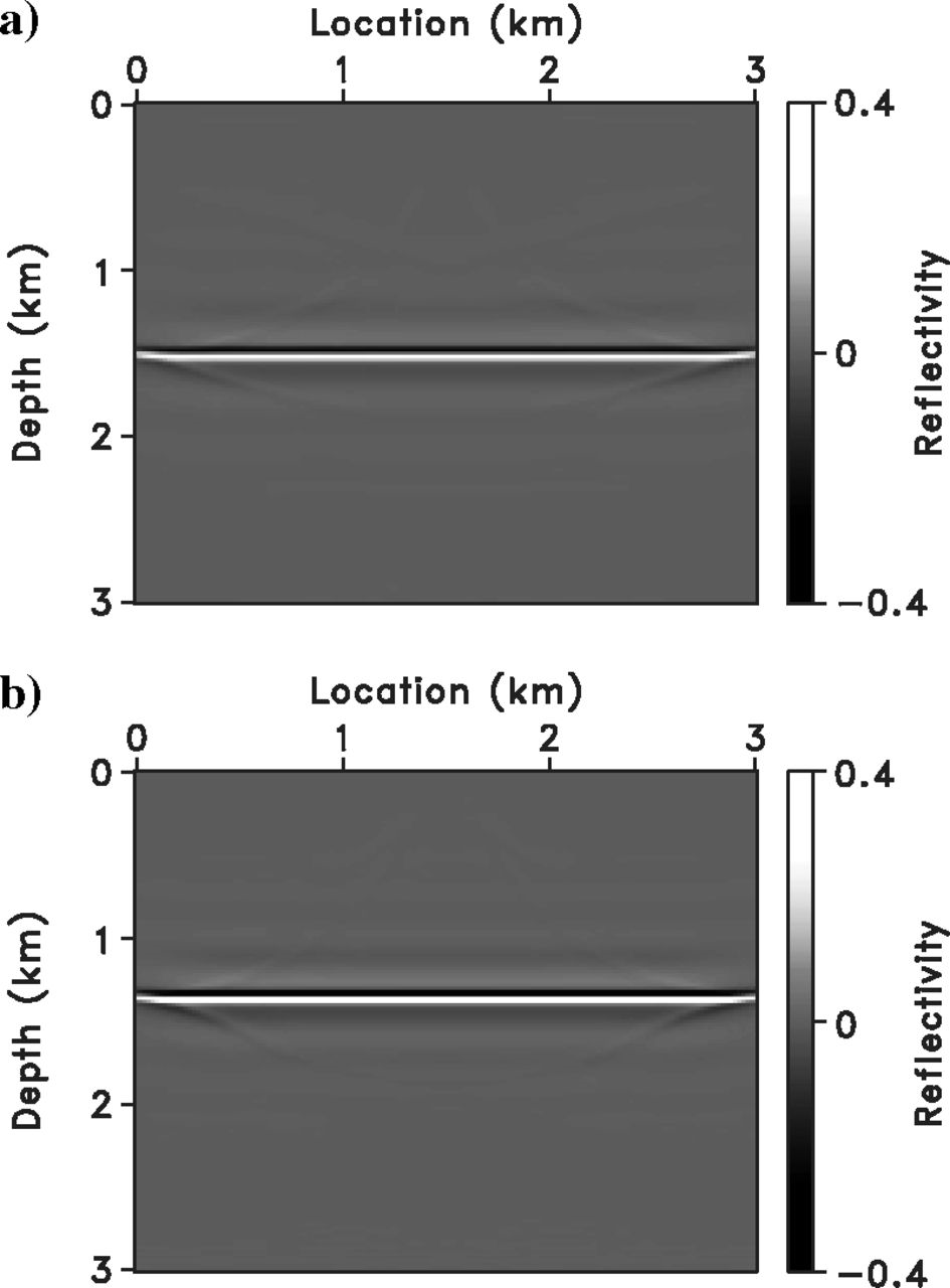
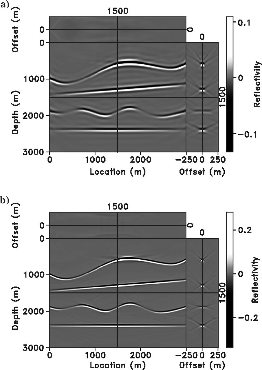
Extended RTM vs. Extended Inversion

Extended RTM image (a) vs. extended inverted reflectivity model (b). The approximate inverse produces correct amplitudes (Hou and Symes 2015).

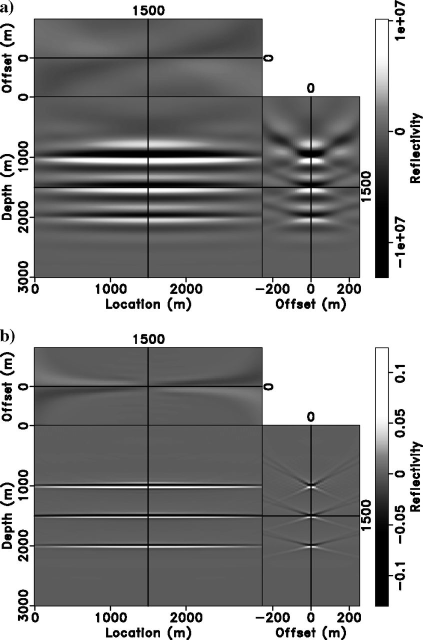
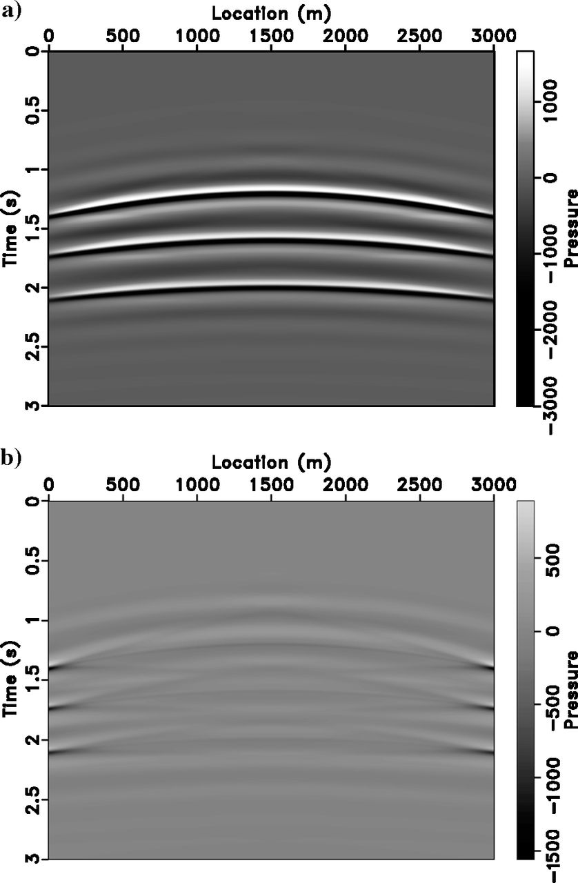
Data Fit Verification

Resimulated data from inverted reflectivity (a) and difference with original data (b). The approximate inverse accurately reproduces the data (Hou and Symes 2015).

Approximate Inverse — Main Result

The approximate inverse to the extended Born modeling operator takes the form (Hou and Symes 2015, Eq. 1):

\[ \bar{F}^\dagger[v_0] = W_{\text{model}}[v_0]\; \bar{F}^*[v_0]\; W_{\text{data}}[v_0] \tag{4}\]

In our LSM lecture notation, this corresponds to left and right preconditioning:

\[ \tilde{\mathbf{m}} = \mathbf{M}_R^{-1}\,\tilde{\mathbf{u}}, \quad \hat{\mathbf{F}} = \mathbf{M}_L^{-1}\,\mathbf{F}\,\mathbf{M}_R^{-1} \]

where:

$W_{\text{data}}[v_0]$ acts as the right preconditioner $\mathbf{M}_L^{-1}$ (applied to data before migration)
$W_{\text{model}}[v_0]$ acts as the left preconditioner $\mathbf{M}_R^{-1}$ (applied to image after migration)

Weight Operators

The weight operators that make $\bar{F}$ approximately unitary (Hou and Symes 2018, Eq. 10):

\[ W_{\text{model}}^{-1} = -8v^4 D_z Q, \qquad W_{\text{data}} = I_t^3\, D_{z_s}\, D_{z_r} \]

where:

$I_t$ = time integration operator
$D_{z_s}, D_{z_r}$ = source and receiver depth derivatives
$D_z$ = depth derivative in image domain
$Q \approx 1$ near $h = 0$ (neglected in practice)

Note

$W_{\text{data}}$ depends only on $v_0$ near sources and receivers — independent of the deep velocity structure. The computational cost of $\bar{F}^\dagger$ is roughly the same as extended RTM. Approximately unitary means that the adjoint is close to the inverse and that most enegry/information is preserved.

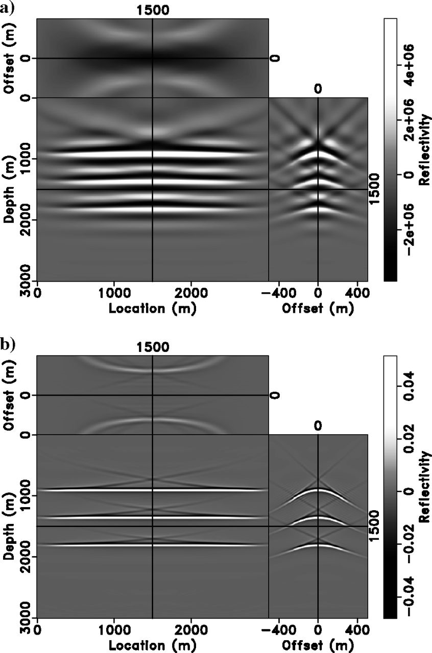
Inversion with Incorrect Velocity

Extended RTM image (a) and extended inverted reflectivity (b) using an **incorrect** background velocity model. The inversion still produces a data-fitting model (Hou and Symes 2015).

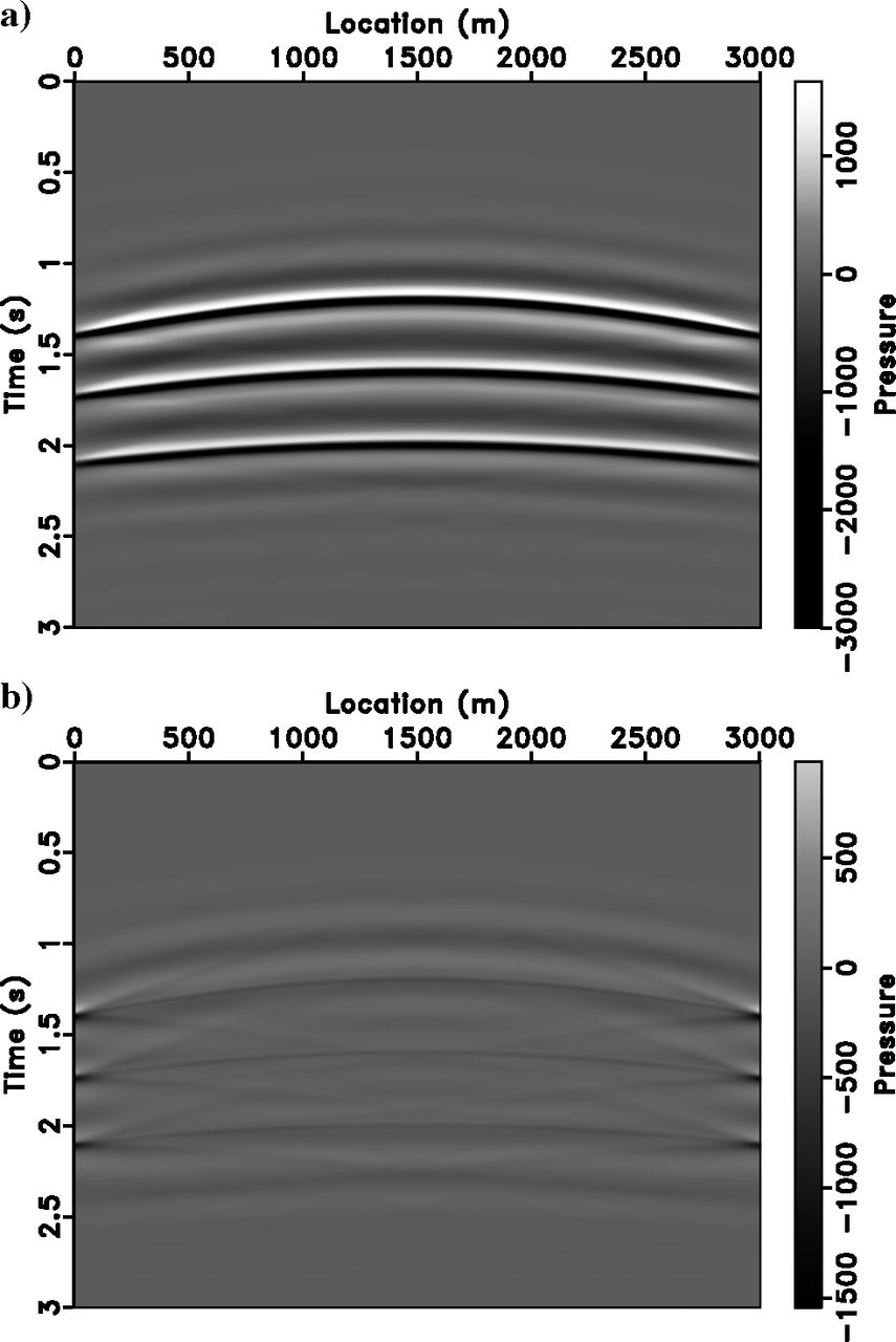
Data Fit with Wrong Velocity

Resimulated data from inverted reflectivity using incorrect velocity (a) and difference with original data (b). Data fit holds even with wrong velocity (Hou and Symes 2015).

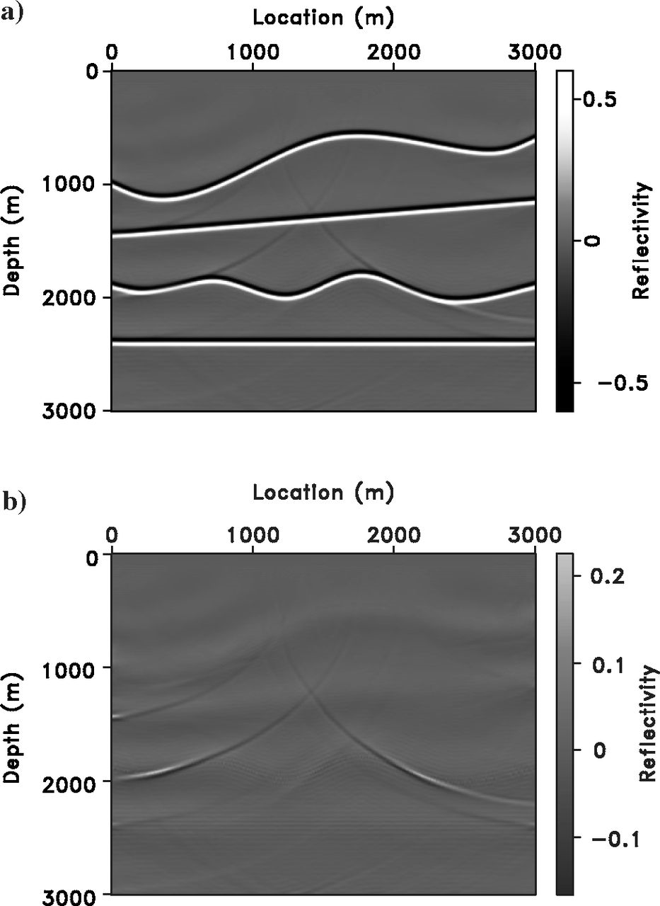
Nonextended Inversion Result

Nonextended inverted reflectivity (stacking over $h$) and difference with original reflectivity model (Hou and Symes 2015).

Gaussian Lens Example

Gaussian lens background velocity model with reflector at 2 km, and corresponding rays and wavefronts (Hou and Symes 2015).

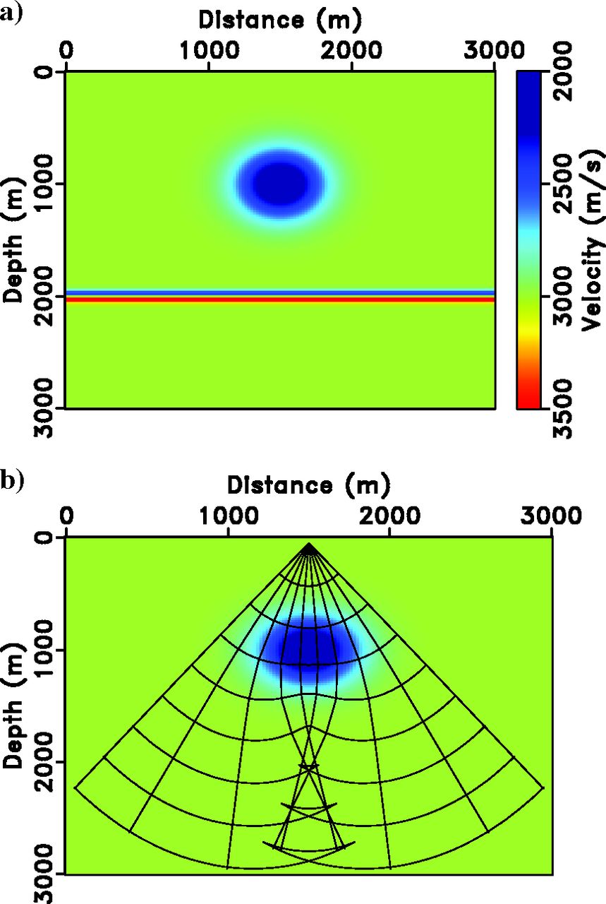
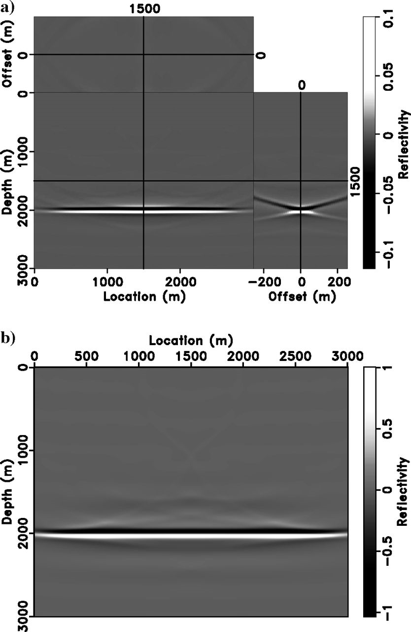
Gaussian Lens — Inversion Results

Extended inverted reflectivity (a) and nonextended inverted reflectivity (b) for the Gaussian lens model (Hou and Symes 2015).

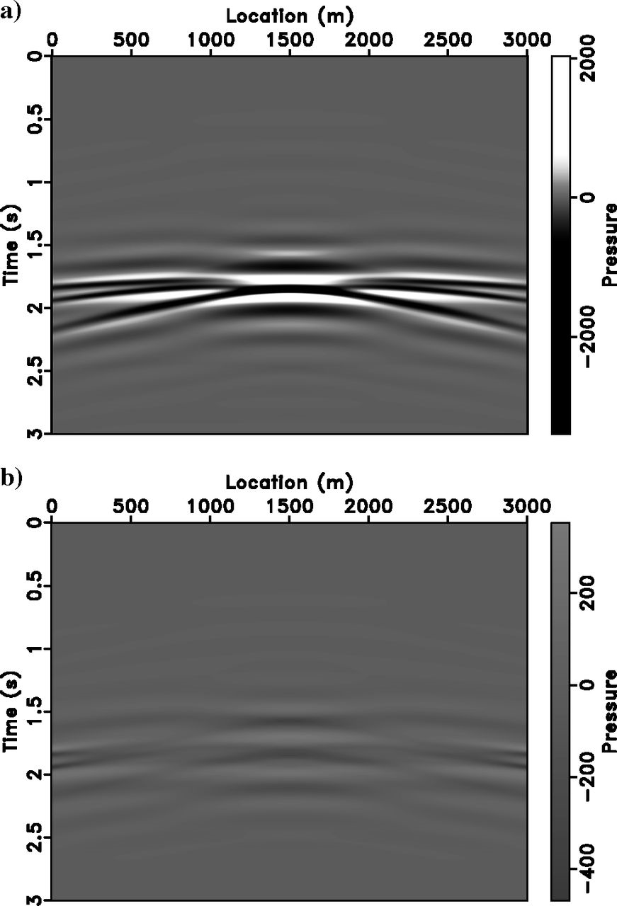
Gaussian Lens — Data Fit

One-shot resimulated Born data (a) and difference with original data (b) for the Gaussian lens model (Hou and Symes 2015).

Extended Least-Squares Migration

Fitting Data with Any Velocity

LSM vs. ELSM — The Key Difference

From our LSM lecture, the least-squares objective is:

\[ J_{\text{LS}} = \frac{1}{2}\|\mathbf{F}\,\delta\mathbf{m} - \delta\mathbf{d}\|^2 \]

Extended LSM replaces $F$ by $\bar{F}$ and $\delta v$ by $\delta\bar{v}(\mathbf{x}, h)$ (Hou and Symes 2016):

\[ J_{\text{ELSM}} = \frac{1}{2}\|\bar{F}[v_0]\,\delta\bar{v} - \delta d\|^2 \]

velocity model extension: $\delta\bar{v}(x,y,h)=\delta v(x,z)\delta(h)$
With the extra offset dimension, the model dimension matches the data dimension
ELSM can fit data with correct or incorrect velocity
Correct velocity $\Rightarrow$ energy focuses at $h = 0$
Incorrect velocity $\Rightarrow$ energy spreads to nonzero $h$, but data is still fit

LSM: Correct vs. Wrong Velocity

Least-squares migration after 30 CG iterations using (a) correct background velocity (2.5 km/s) and (b) incorrect background velocity (2 km/s) (Hou and Symes 2016). The wrong velocity image is wronly positioned and has incorrect amplitudes.

ELSM: Correct vs. Wrong Velocity

Extended least-squares migration after 30 CG iterations using (a) correct velocity (2.5 km/s) and (b) incorrect velocity (2 km/s). Offset range: $[-500, 500]$ m (correct) and $[-1000, 1000]$ m (wrong) (Hou and Symes 2016).

Tip

With incorrect velocity, the image is not focused at $h = 0$ but the data is still fit. The offset range must be larger to accommodate the velocity error.

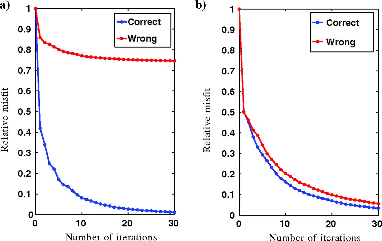
Convergence: LSM vs. ELSM

Relative data misfit for (a) LSM and (b) ELSM with correct (blue) and wrong (red) velocity. ELSM residual converges to zero with both velocities (Hou and Symes 2016).

Weighted Conjugate Gradient

Accelerating ELSM Convergence

The Unitarity Property

Because $\bar{F}^\dagger \bar{F} \approx I$ (the extended Born operator is approximately unitary w.r.t. weighted norms), CG with weighted norms converges dramatically faster (Hou and Symes 2016).

The weighted CG uses inner products:

\[ \langle \delta\bar{v}_1, \delta\bar{v}_2 \rangle_{\text{model}} = \sum_{x,z,h} \delta\bar{v}_1(x,z,h)\,(W_{\text{model}}\,\delta\bar{v}_2)(x,z,h) \]

\[ \langle d_1, d_2 \rangle_{\text{data}} = \sum_{s,r,t} d_1(\mathbf{x}_s, \mathbf{x}_r, t)\,(W_{\text{data}}\, d_2)(\mathbf{x}_s, \mathbf{x}_r, t) \]

Algorithm: Weighted Conjugate Gradient

Algorithm 1 from Hou and Symes (2016). Inputs: operators $\bar{F}$, $\bar{F}^\dagger$, data $\delta d$, initial estimate $\delta\bar{v}_0$.

$z_0 \leftarrow \bar{F}^\dagger(\delta d - \bar{F}\,\delta\bar{v}_0)$
$p_0 \leftarrow z_0$, $\quad k \leftarrow 0$
repeat
$\quad \alpha_k \leftarrow \dfrac{\langle z_k, z_k \rangle_{\text{model}}}{\langle \bar{F}\,p_k, \bar{F}\,p_k \rangle_{\text{data}}}$
$\quad \delta\bar{v}_{k+1} \leftarrow \delta\bar{v}_k + \alpha_k\, p_k$
$\quad z_{k+1} \leftarrow z_k - \alpha_k\, \bar{F}^\dagger \bar{F}\, p_k$
$\quad \beta_{k+1} \leftarrow \dfrac{\langle z_{k+1}, z_{k+1} \rangle_{\text{model}}}{\langle z_k, z_k \rangle_{\text{model}}}$
$\quad p_{k+1} \leftarrow z_{k+1} + \beta_{k+1}\, p_k$
$\quad k \leftarrow k + 1$
until convergence

Note

Each iteration costs roughly the same as standard CG — one demigration ($\bar{F}$) and one migration ($\bar{F}^\dagger$). The weights add negligible cost.

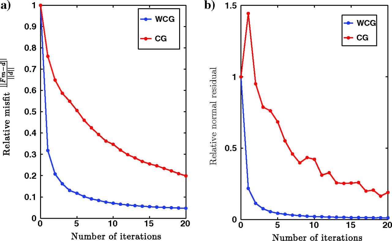
Simple Model — CG vs. WCG

Simple layered model. (a) Background velocity model and (b) reflectivity model (Hou and Symes 2016).

ELSM Results — CG vs. WCG

Twenty iterations of ELSM via (a) CG and (b) WCG iteration. WCG converges dramatically faster (Hou and Symes 2016).

Physical Image from WCG

Physical image from stacking 20 WCG iterations along subsurface offset (a), and difference with original reflectivity (b). Same gray scale (Hou and Symes 2016).

Marmousi Examples

Testing on a Realistic Model

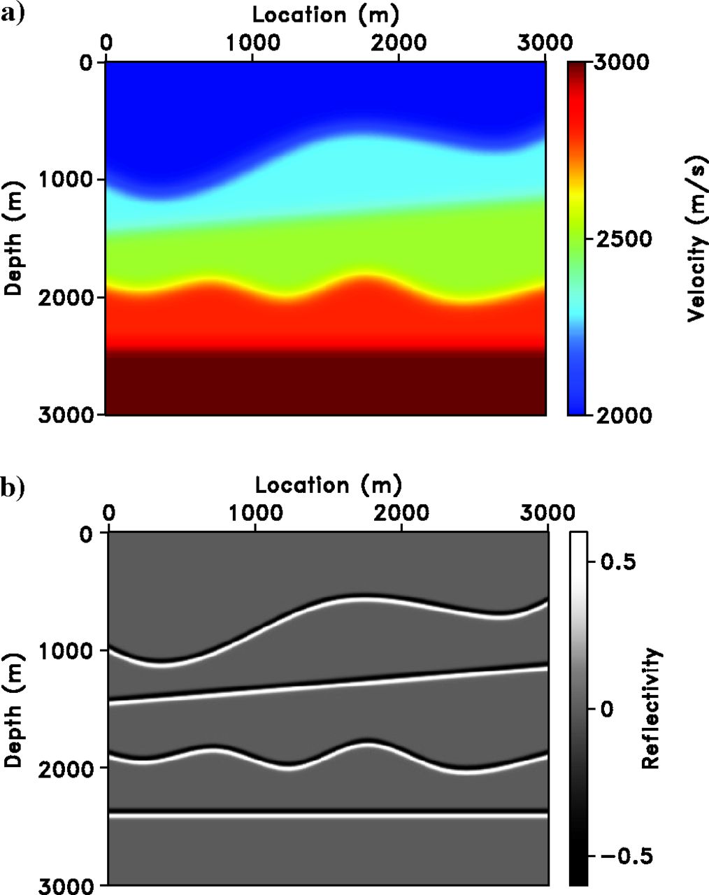
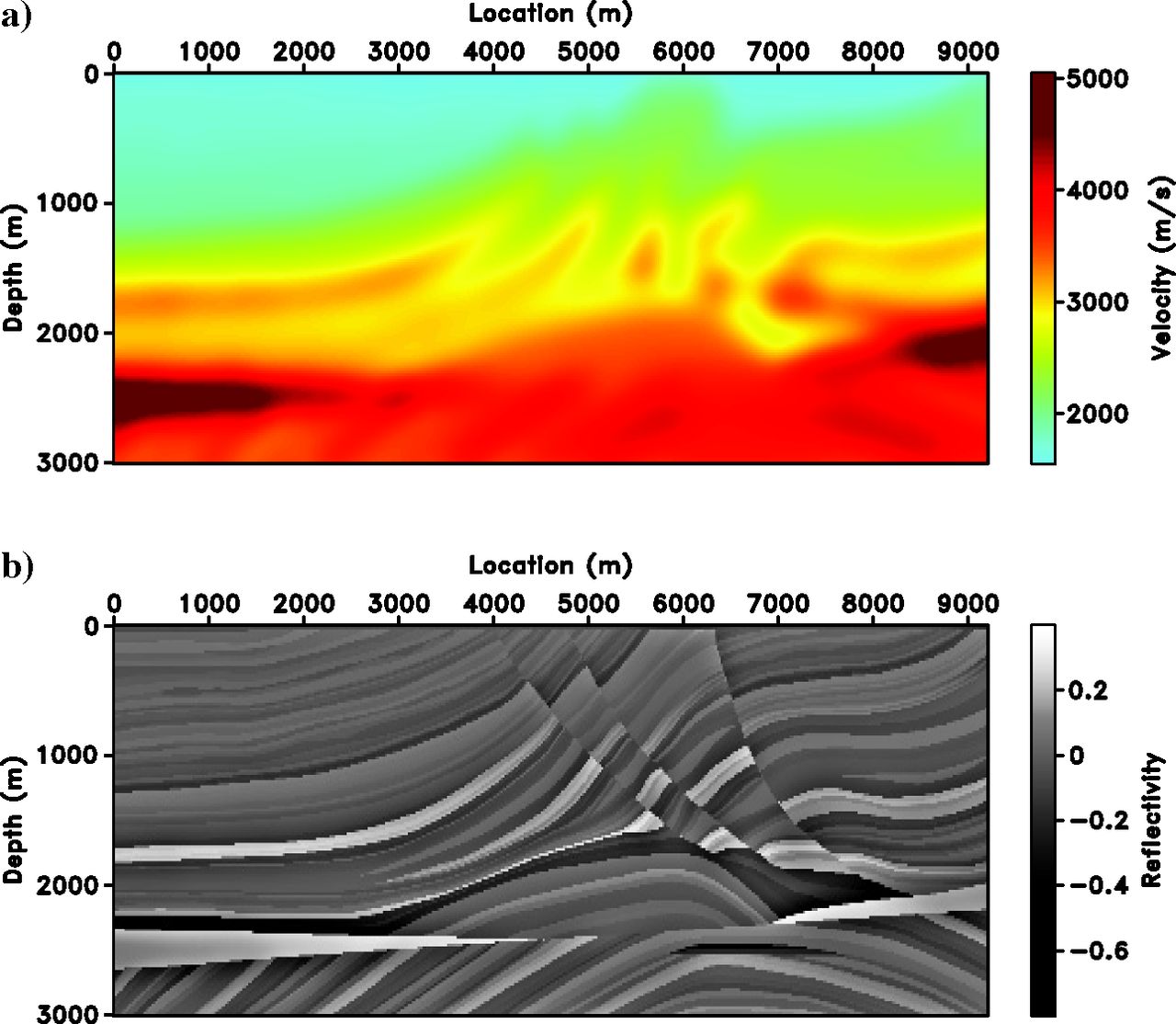
Marmousi Model Setup

Marmousi model. (a) Background velocity obtained by smoothing the original model, and (b) reflectivity model (difference between original and smoothed) (Hou and Symes 2016).

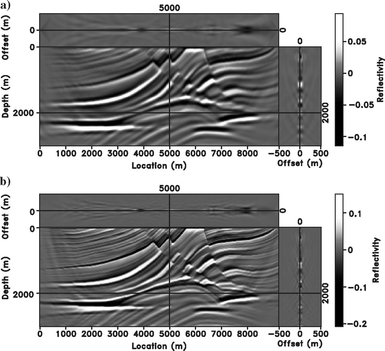
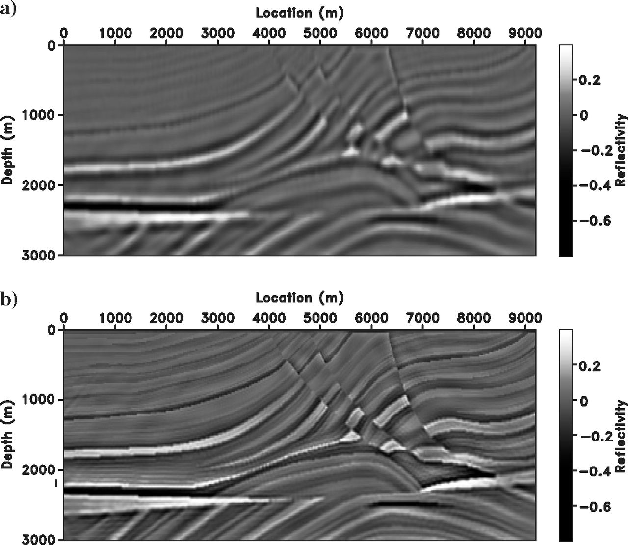
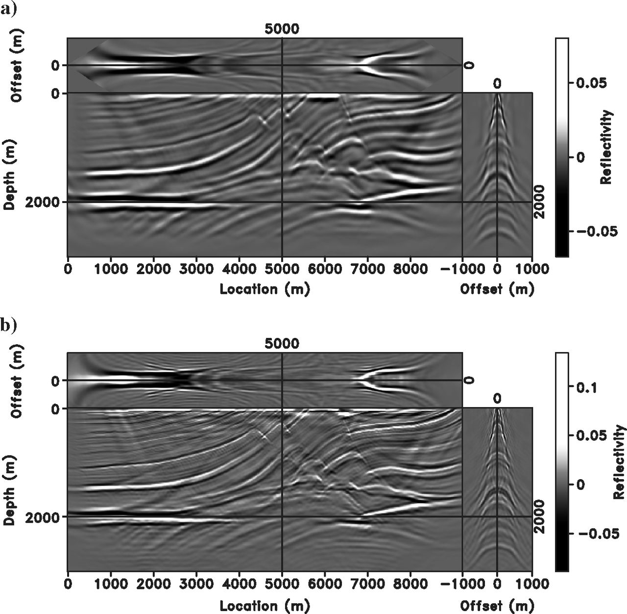
Marmousi — ELSM Results

Twenty iterations of ELSM via (a) CG and (b) WCG iteration on the Marmousi model. WCG yields noticeably higher resolution (Hou and Symes 2016).

Marmousi — Stacked Images

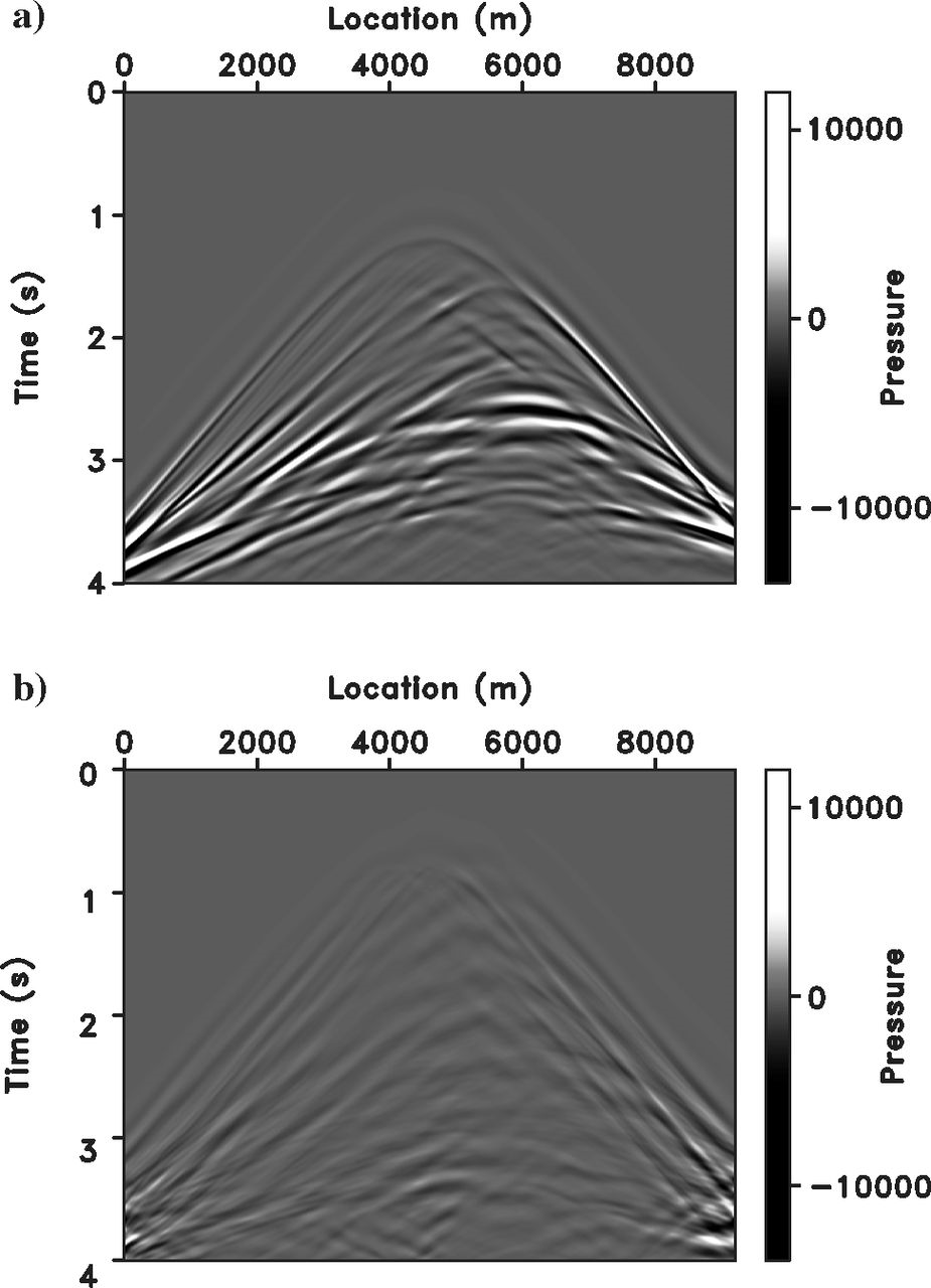
Physical images from stacking along offset: (a) 20 CG iterations and (b) 20 WCG iterations. WCG produces a higher-resolution result (Hou and Symes 2016).

Marmousi — Data Fit

Single-shot Born data at 5 km (a) and data residual ($\times 10$) after 20 WCG iterations (b). The data is accurately reconstructed (Hou and Symes 2016).

Tip

The residual is amplified by a factor of 10 — the actual misfit is very small, confirming accurate data fit.

Marmousi — Wrong Velocity

Twenty iterations of ELSM via (a) CG and (b) WCG with incorrect velocity (0.9 × true). Energy spreads to nonzero offset but data is still fit (Hou and Symes 2016).

Important

The image is not focused for the poor background velocity, yet data is fit (as in Figure 14). The offset range must be doubled ($[-1000, 1000]$ m) to accommodate the velocity error. This is the key feature exploited for velocity analysis.

Marmousi — Convergence Comparison

Relative data misfit (a) and relative normal residual (b) for CG (red) and WCG (blue) with incorrect velocity. WCG converges faster even with velocity error (Hou and Symes 2016).

Note

The convergence behavior with wrong velocity is very similar to the correct velocity case — WCG acceleration is robust to velocity error.

DSO Velocity Analysis

Differential Semblance Optimization

DSO Objective Function

In the subsurface-offset domain, the semblance condition requires a focused offset gather. The DSO objective penalizes energy at nonzero offset (Hou and Symes 2018, Eq. 11):

\[ J[v] = \frac{1}{2}\|h\, I(\mathbf{x}, h)\|^2 \tag{5}\]

where $I(\mathbf{x}, h)$ is the extended image from either RTM ($\bar{F}^*$) or the approximate inverse ($\bar{F}^\dagger$).

Minimization penalizes energy outside $h = 0$ $\Rightarrow$ focuses the gather
Focused gather implies correct velocity
This is the basic idea of DSO-based velocity analysis

RTM vs. Inversion — Objective Function

Normalized objective function: MVA with RTM (red), MVA + stack power (green), and IVA with approximate inverse (blue). Velocity ranges from 2 to 3 km/s. True velocity is 2.5 km/s (Hou and Symes 2018).

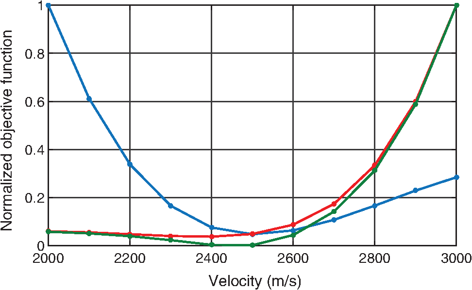
Critical observation

The MVA objective (red) has its minimum shifted to 2400 m/s — the wrong velocity! The IVA objective (blue) correctly minimizes at 2500 m/s. The so-called “gradient artifacts” are actually a problem of the objective function, not the gradient.

Velocity Update Results

(a) True model, (b) initial model, 50-iteration L-BFGS result for (c) the adjoint operator (MVA), and (d) the approximate inverse operator (IVA) (Hou and Symes 2018).

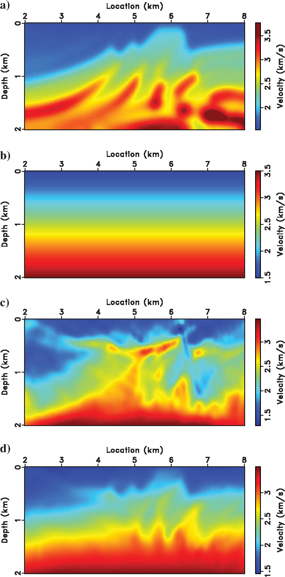
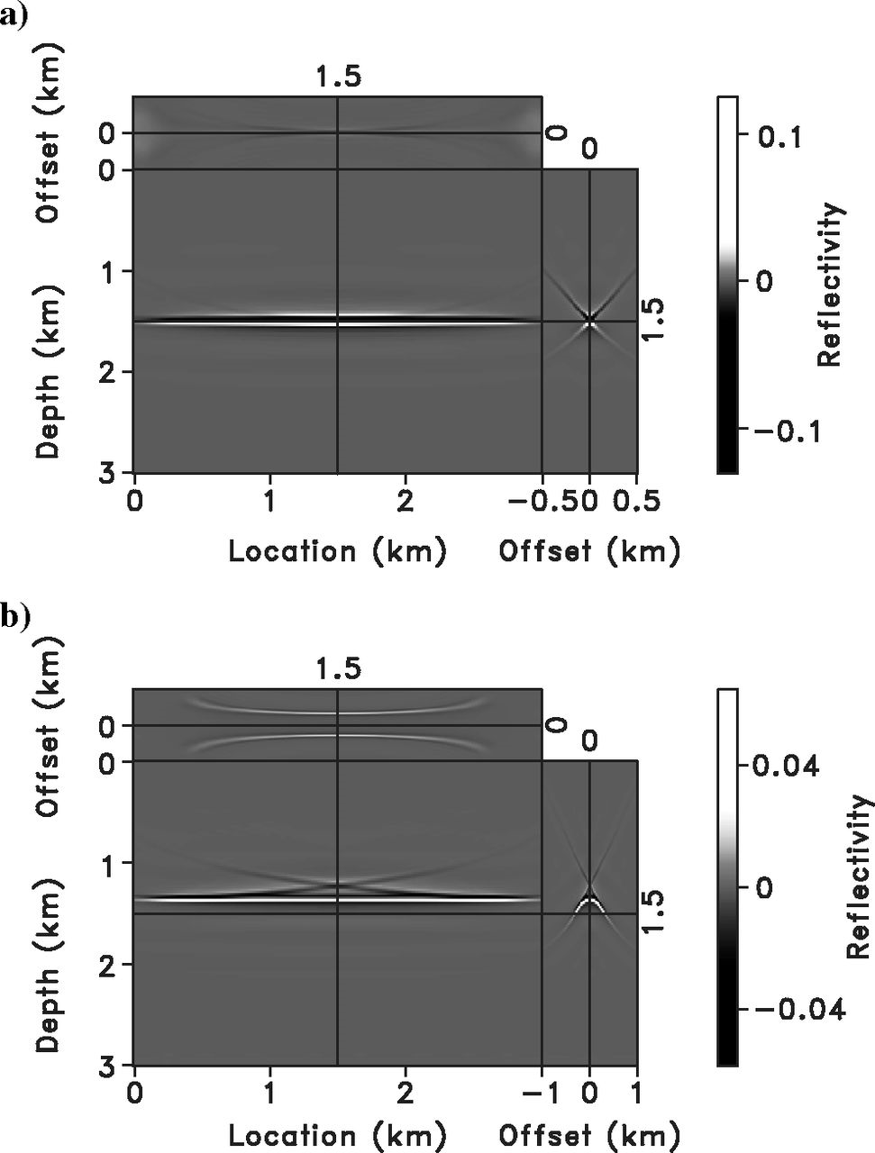
Zero-Offset Images — Velocity Quality

Zero-offset approximate inverse image associated with different velocity models from the velocity update (Hou and Symes 2018).

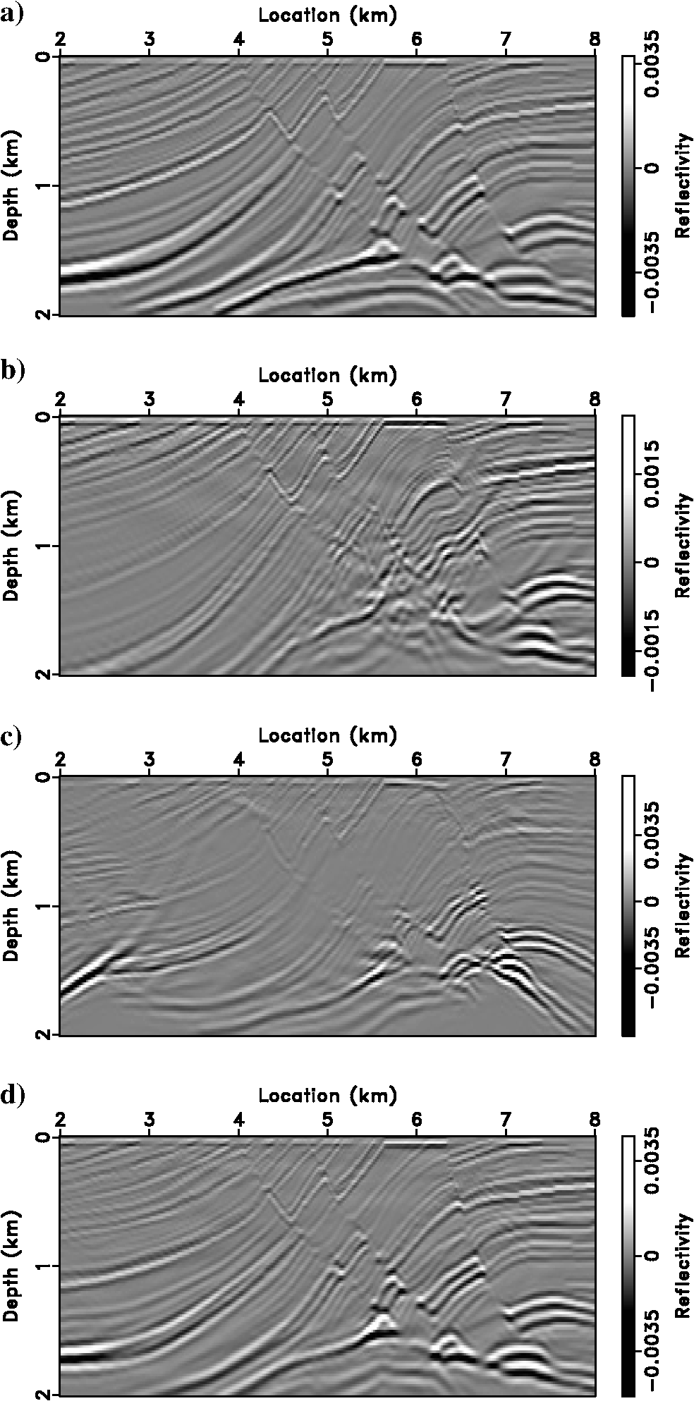
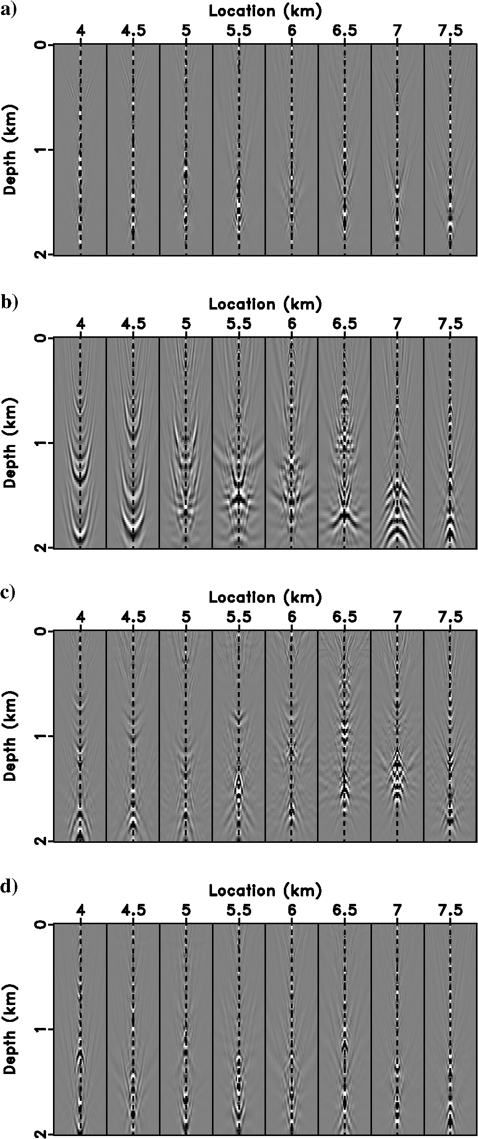
Image Gathers — Focusing Quality

Approximate inverse image gathers in the subsurface-offset domain corresponding to the images above. Focused gathers confirm improved velocity (Hou and Symes 2018).

What Goes Wrong?

Artifacts and Limitations of WEMVA

The Artifact Problem

When RTM (the adjoint) is used instead of inversion, artifacts corrupt the velocity update (Hou and Symes 2018):

RTM offset gathers show noise at nonzero offset (red arrows). This noise is due to incorrect, dip-dependent amplitudes in migrated images that cannot interfere destructively (Hou and Symes 2018).

Fundamental Limitations of WEMVA

Problems with Wave-Equation MVA

Despite the improvements from using the approximate inverse, WEMVA has fundamental issues:

Strong reflectors dominate the objective — The DSO objective $J = \frac{1}{2}\|h\,I(\mathbf{x},h)\|^2$ is weighted toward high-amplitude events, which may not carry the best velocity information
Fails with strong multiples — Surface-related or internal multiples violate the single-scattering (Born) assumption, corrupting the image gathers and biasing the velocity update
Requires extensive hand-holding — Dip filtering, offset range selection, regularization, and balancing of DSO vs. stack-power terms all require manual tuning
Limited physics — The constant-density acoustic approximation and idealized 2D acquisition geometry are restrictive

The road ahead

These limitations motivate the transition to full-waveform inversion (FWI), which directly fits the data without requiring image-domain proxies. FWI will be the subject of our next lectures.

Summary

Subsurface-offset extension adds degrees of freedom to match data and model dimensions
Extended imaging (RTM or approximate inverse) produces offset gathers $I(\mathbf{x}, h)$
Focusing at $h = 0$ indicates correct velocity; unfocused gathers indicate velocity error
The approximate inverse $\bar{F}^\dagger = W_{\text{model}}\,\bar{F}^*\,W_{\text{data}}$ is critical — using RTM alone leads to artifacts in velocity analysis
Weighted CG dramatically accelerates extended LSM convergence
DSO provides a smooth, unimodal objective for velocity updates (when using inversion, not adjoint)
WEMVA has fundamental limitations: strong reflectors, multiples, hand-holding
Next: Full-waveform inversion — a more direct approach to velocity estimation

Key Takeaway

From image volumes to FWI

The main goal of subsurface-offset image volumes is to obtain estimates for the background velocity model $v_0$. While WEMVA with the approximate inverse improves upon classical MVA, its fundamental limitations (dominance of strong reflectors, sensitivity to multiples, need for hand-holding) motivate the move to full-waveform inversion, which we cover next.

We leave the directional scattering aspect (AVA/AVP from image gathers) for a later lecture.

References

Claerbout, Jon F. 1985. Imaging the Earth’s Interior. Blackwell Scientific Publishers.

Hou, Jie, and William W. Symes. 2015. “An Approximate Inverse to the Extended Born Modeling Operator.” Geophysics 80 (6): R331–49. https://doi.org/10.1190/geo2014-0592.1.

———. 2016. “Accelerating Extended Least-Squares Migration with Weighted Conjugate Gradient Iteration.” Geophysics 81 (4): S165–79. https://doi.org/10.1190/geo2015-0499.1.

———. 2018. “Inversion Velocity Analysis in the Subsurface-Offset Domain.” Geophysics 83 (2): R189–200. https://doi.org/10.1190/geo2017-0059.1.

Symes, William W. 2008. “Migration Velocity Analysis and Waveform Inversion.” Geophysical Prospecting 56: 765–90. https://doi.org/10.1111/j.1365-2478.2008.00698.x.

Continuous (Papers)	Discrete (Lecture A)
\(F[v_0]\,\delta v = \delta d\)	\(\mathbf{F}\,\delta\mathbf{m} = \delta\mathbf{d}\)
\(G(\mathbf{x}_s, \mathbf{x}, t)\)	\(\mathbf{A}^{-1}(\mathbf{m})\,\mathbf{q}_s\)
\(F^*[v_0]\,\delta d\) (RTM)	\(\mathbf{F}^T\,\delta\mathbf{d}\) (adjoint)
Imaging condition	\([\nabla_\mathbf{m} J]_i = \sum_s \sum_k v_s(x_i,t_k)\,\ddot{u}_s(x_i,t_k)\,\Delta t\)