Linearized AVO Inversion
Quantitative Interpretation of Seismic Amplitudes
2026-02-25


Linearized AVO Inversion
Quantitative Interpretation of Seismic Amplitudes
Felix J. Herrmann
School of Earth & Atmospheric Sciences — Georgia Institute of Technology
Slides are adapted from Eric Verschuur
Impedance Inversion with a Background
Approach: start with a low-frequency background model \(\mathbf{m}_0\) and solve for perturbations \(\delta\mathbf{m}\):
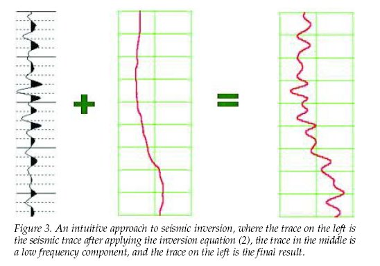
The low-frequency background comes from well logs or velocity analysis, and the band-limited perturbation is inverted from the seismic data.
Application: Marlin Field (Gulf of Mexico)
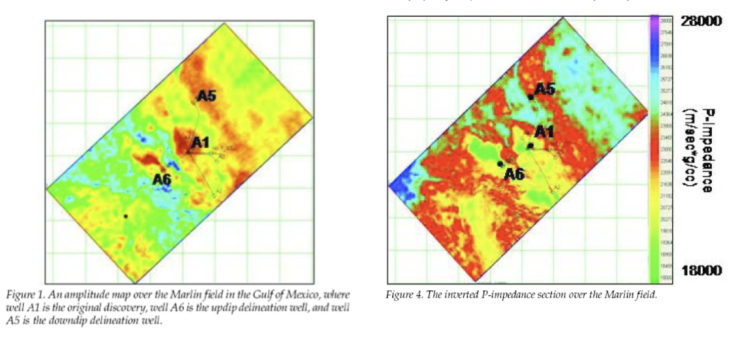
Inverted P-impedance section over the Marlin Field, Gulf of Mexico.
- All wells correlate with amplitude anomalies
- Impedance inversion reveals gas-bearing zones at A1 and A6. Why?
- From Russell, Hampson, and Bankhead (2006)
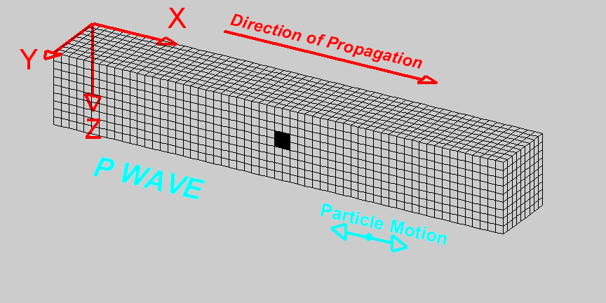
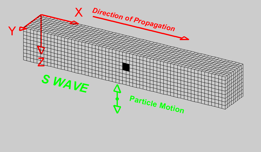
Bulk & Shear Modulus, P- & S-Wave Speeds
The elastic medium is characterized by density \(\rho(\mathbf{r})\), bulk modulus \(K(\mathbf{r})\), and shear modulus \(\mu(\mathbf{r})\).
Compressional (P-wave) velocity:
\[ \alpha = c_P = \sqrt{\frac{K + \frac{4}{3}\mu}{\rho}} = \sqrt{\frac{\lambda + 2\mu}{\rho}} \]
Shear (S-wave) velocity:
\[ \beta = c_S = \sqrt{\frac{\mu}{\rho}} \]
Snell’s Law and Mode Conversion
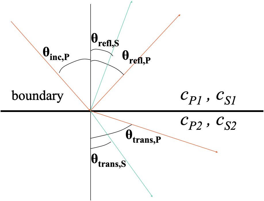
An incident P-wave at a solid-solid interface generates four waves:
- Reflected P-wave (angle \(\theta_{P1}^{\text{refl}}\))
- Reflected S-wave (angle \(\theta_{S1}^{\text{refl}}\))
- Transmitted P-wave (angle \(\theta_{P2}^{\text{trans}}\))
- Transmitted S-wave (angle \(\theta_{S2}^{\text{trans}}\))
All angles are related through Snell’s law via the common ray parameter \(p\).
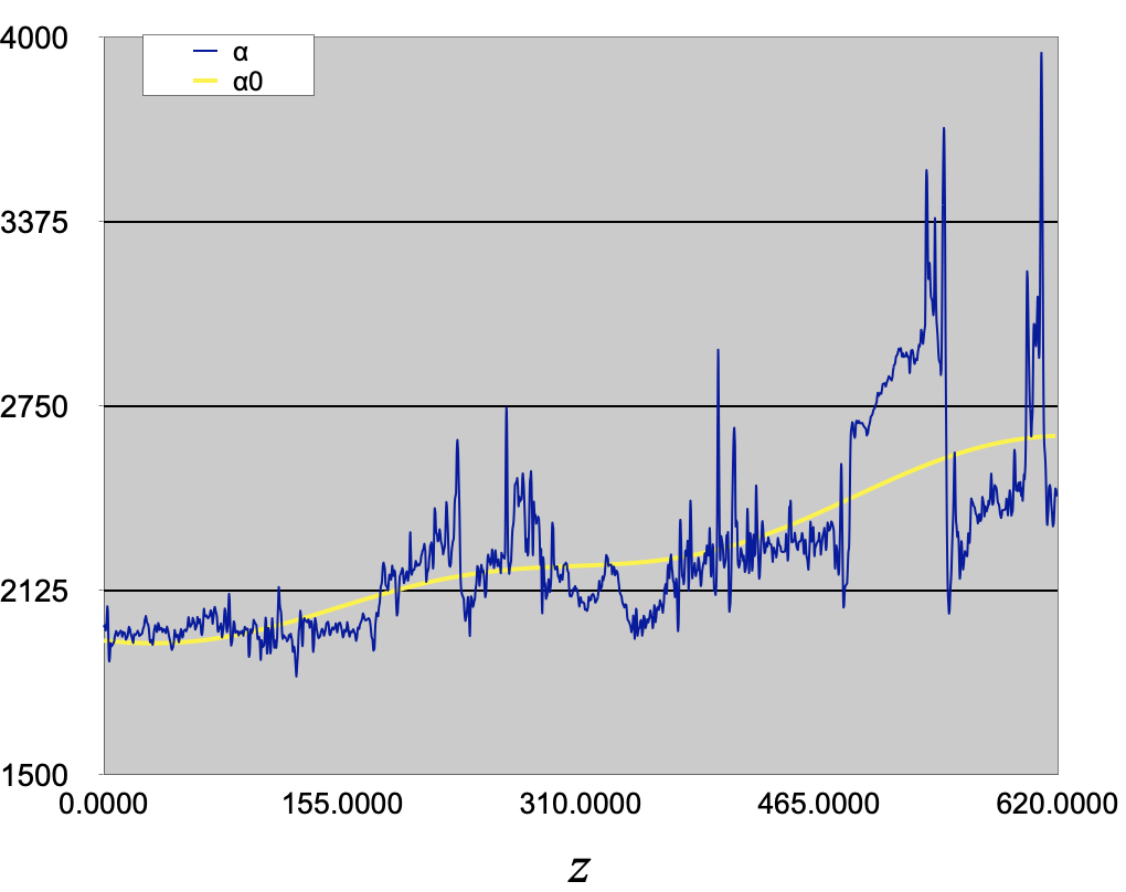
Well \(c_p\) + smoothed well
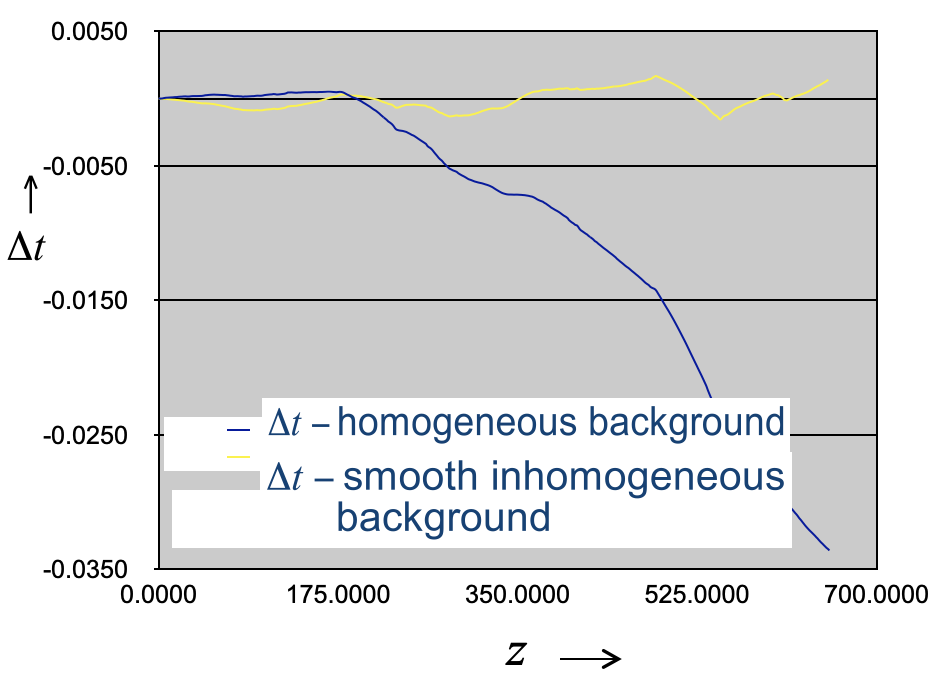
Traveltimes
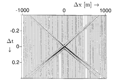
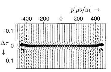
The Linear Radon Transform
The linear Radon transform (\(\tau\)-\(p\) transform) maps data from the \(x\)-\(t\) domain to the \(\tau\)-\(p\) domain:
\[ m(p, \tau) = \int_{-\infty}^{+\infty} d(x, t = \tau + px)\,dx \]
![]()
![]()
One point in the Radon domain \(m(p,\tau)\) is obtained by stacking the input data along a straight line \(t = \tau + px\).
Radon Amplitudes and Reflection Coefficients
After back-propagation and Radon transform, the focused amplitudes approximate the plane-wave reflection coefficient:
Note
After back-propagation, the focused point in \(x\)-\(t\) maps to a focused point in \(\tau\)-\(p\), where the amplitudes approximate the reflection coefficients \(R_i(p)\) convolved with a stretched wavelet (Wijngaarden 1998).
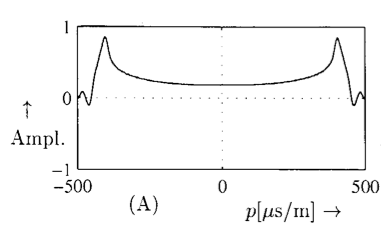
Shot data and migrated data in \((\tau-p)\)
After Wijngaarden (1998)
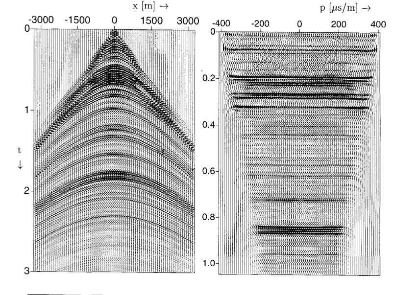
Inversion results
Left: after migration and Radon. Right: inverted contrasts
Synthetic Example: 1.5D Layered Model
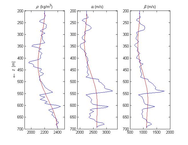
Horizontally layered model with smooth curves representing the background model.
. . .
- Source: zero-phase wavelet with realistic bandwidth
- Inversion in the \(\tau\)-\(p\) domain
- Compare predicted vs. actual properties
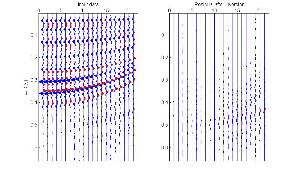
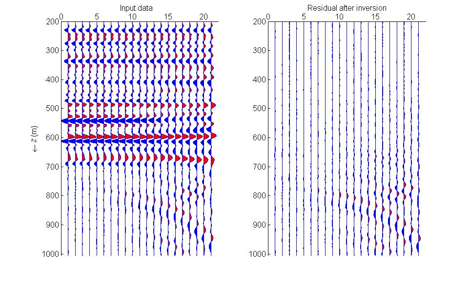
Data + residual time & imaged domain
Time-domain
Imaged domain
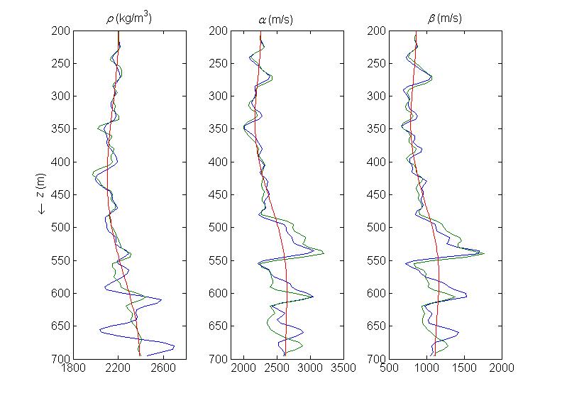
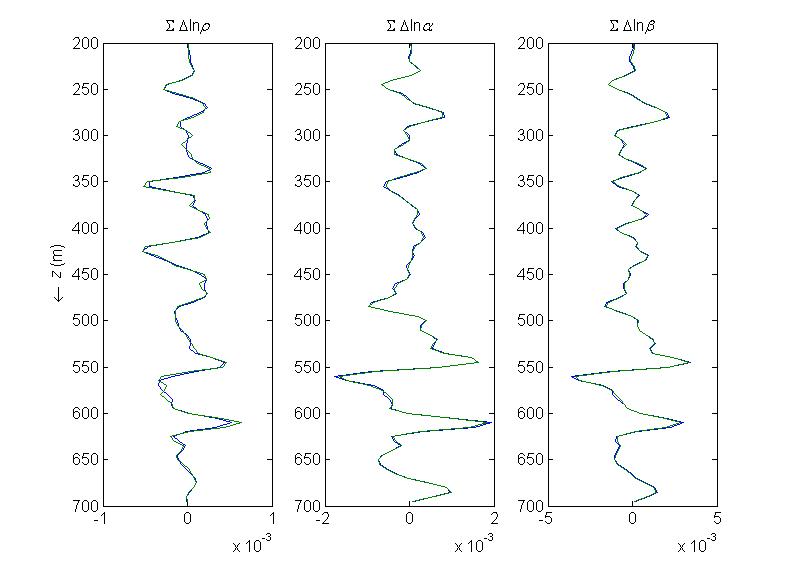
Band-Limited vs. Broadband Inversions
Band-limited result
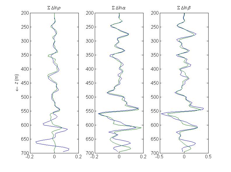
Predicted (green) vs. actual (blue) band-limited log properties. Spatial band-limitation is derived from the source wavelet.
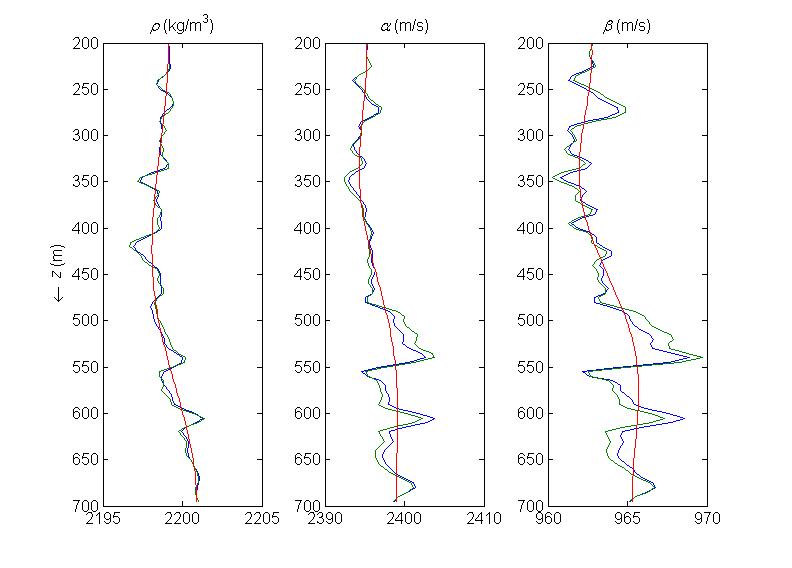
Broadband result
Adding band-limited predictions to background values. Note discrepancies due to the spectral gap.
The Spectral Gap
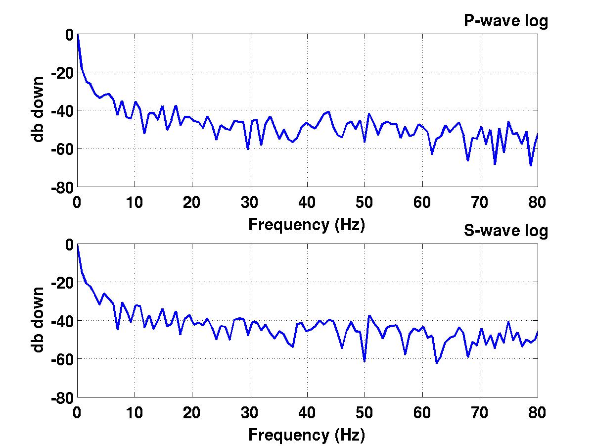
With linear imaging we cannot bridge the spectral gap between:
- The low-frequency content of the background model
- The band-limited seismic amplitudes
. . .
The gap arises because the seismic wavelet has no energy at very low frequencies.
. . .
Important
Only nonlinear inversion (e.g., with a sparseness constraint) or additional information (well logs) can bridge this gap.
Low-Contrast Validation — Model & Data
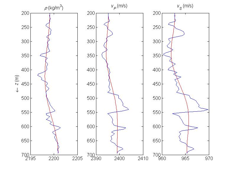
Low-contrast model (0.01\(\times\) real contrasts) with \(\rho\), \(v_P\), \(v_S\) vs. depth. Smooth red curves show the background model.
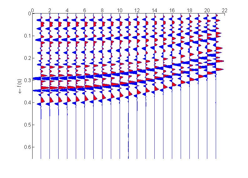
\(\tau\)-\(p\) Radon-domain data for the low-contrast model, showing the amplitude-versus-ray-parameter variation.
Low-Contrast Validation — Inversion Results
For very low contrasts (0.01\(\times\) real), the linearized inversion performs excellently — validating the method.
Even with near-perfect linear inversion, the spectral gap still causes discrepancies in the broadband result.
Real Data Example
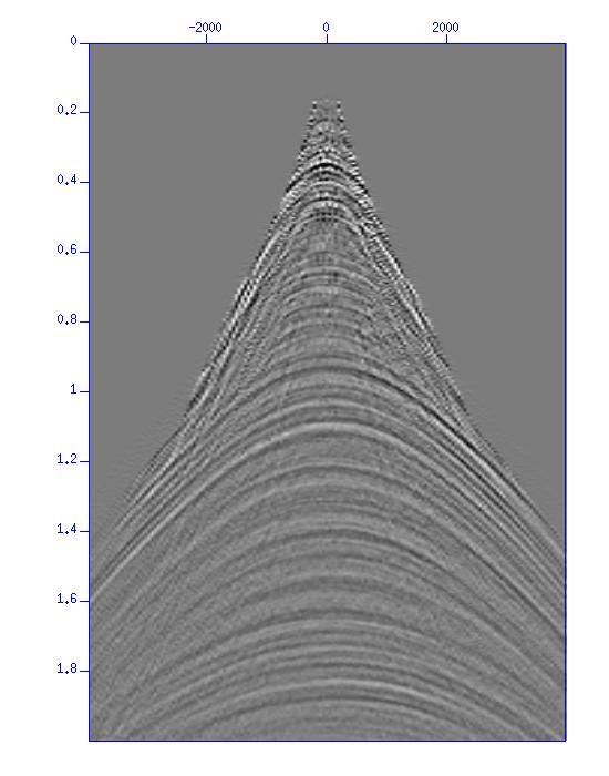
Input processed surface shot record and stacked section.
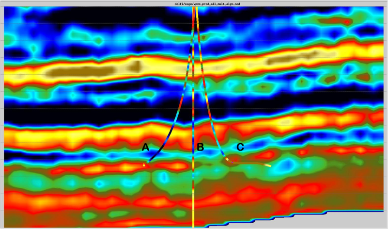
Linear elastic inversion results of redatumed data at top of target interval. (MSc thesis work by Xander Staal)
This lecture was prepared with the assistance of Claude (Anthropic) and validated by Felix J. Herrmann.
This work is licensed under a Creative Commons Attribution-NonCommercial-ShareAlike 4.0 International License.
