Convolution — continuous
Let \(w(t)\) denote the source wavelet and \(r(t)\) the reflectivity series. Their convolution is
\[
d(t) = (w \ast r)(t) = \int_{-\infty}^{\infty} w(\tau)\, r(t - \tau)\, d\tau
\]
where \(d(t)\) is the recorded seismic trace.
Physical interpretation: the output \(d(t)\) is a weighted superposition of shifted copies of \(r(t)\), with weights given by \(w(\tau)\).
Correlation — as adjoint of convolution
The cross-correlation of \(w(t)\) with \(d(t)\) is
\[
r_{wd}(\tau) = \int_{-\infty}^{\infty} w(t)\, d(t + \tau)\, dt
\]
This is equivalently written as convolution with the time-reversed wavelet:
\[
r_{wd}(\tau) = (w(-\cdot) \ast d)(\tau)
\]
In operator language, correlation is the adjoint (transpose) of convolution: if \(\mathbf{d} = \mathbf{W}\mathbf{r}\), then \(\mathbf{W}^T\mathbf{d}\) computes the cross-correlation between the wavelet and the seismic trace.
The auto-correlation is the special case: \(r_{ww}(\tau) = \int w(t)\, w(t + \tau)\, dt\).
Fourier-domain view
Let \(W(f)\), \(R(f)\), \(D(f)\) denote the Fourier transforms of \(w(t)\), \(r(t)\), \(d(t)\). Then:
Convolution in time becomes multiplication in frequency:
\[
D(f) = W(f)\, R(f)
\]
Cross-correlation becomes
\[
R_{wd}(f) = W^*(f)\, D(f)
\]
Auto-correlation becomes
\[
R_{ww}(f) = |W(f)|^2
\]
where \(W^*(f)\) denotes the complex conjugate of \(W(f)\).
Discrete convolution
For sampled signals \(w[n]\) and \(r[n]\) with sampling interval \(\Delta t\):
\[
d[n] = \sum_{k} w[k]\, r[n - k]
\]
Convolution is a linear operation, which can be written in matrix form:
\[
\mathbf{d} = \mathbf{W}\, \mathbf{r}
\]
where \(\mathbf{W}\) is a Toeplitz matrix built from the wavelet samples. Its adjoint \(\mathbf{W}^T\) computes correlation.
Discrete Fourier-domain equivalence
Let \(\mathbf{F}\) denote the DFT matrix. Then \(\hat{\mathbf{d}} = \mathbf{F}\mathbf{d}\) and the convolution becomes an elementwise (Hadamard) product:
\[
\hat{\mathbf{d}} = \hat{\mathbf{w}} \odot \hat{\mathbf{r}} = \operatorname{diag}(\hat{\mathbf{w}})\, \hat{\mathbf{r}}
\]
where \(\hat{\mathbf{W}} = \mathbf{F}\mathbf{w}\), \(\hat{\mathbf{R}} = \mathbf{F}\mathbf{r}\), and \(\odot\) is the Hadamard (elementwise) product.
This means convolution is diagonalized by the DFT — each frequency is independent.
Seismic convolutional model
The 1-D seismic trace is modeled as
\[
d(t) = w(t) \ast r(t) + n(t)
\]
where:
- \(w(t)\) — source wavelet, the band-limited pulse emitted by the seismic source
- \(r(t)\) — reflectivity series, a sequence of spikes at impedance boundaries
- \(n(t)\) — additive noise (ambient, instrumental, etc.)
- \(d(t)\) — recorded seismogram
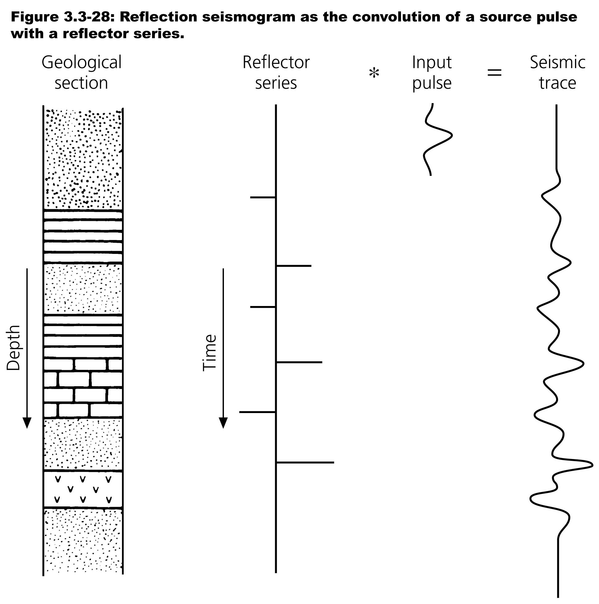
Convolutional model — geological picture
![]()
Geological section \(\to\) impedance contrasts \(\to\) reflectivity series \(r(t)\) convolved with source wavelet \(w(t)\) yields the seismic trace \(d(t)\). (Yilmaz 2001)
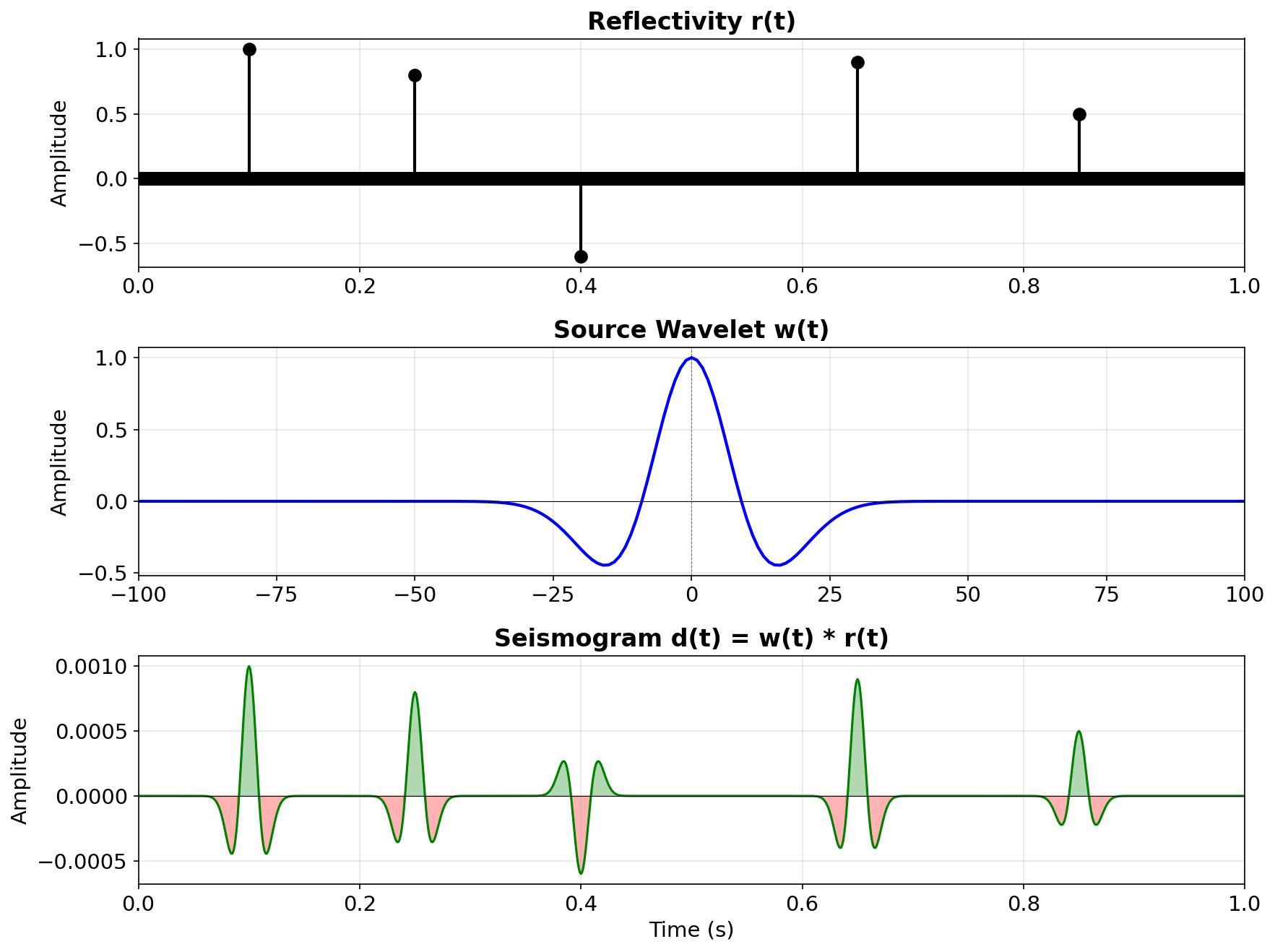
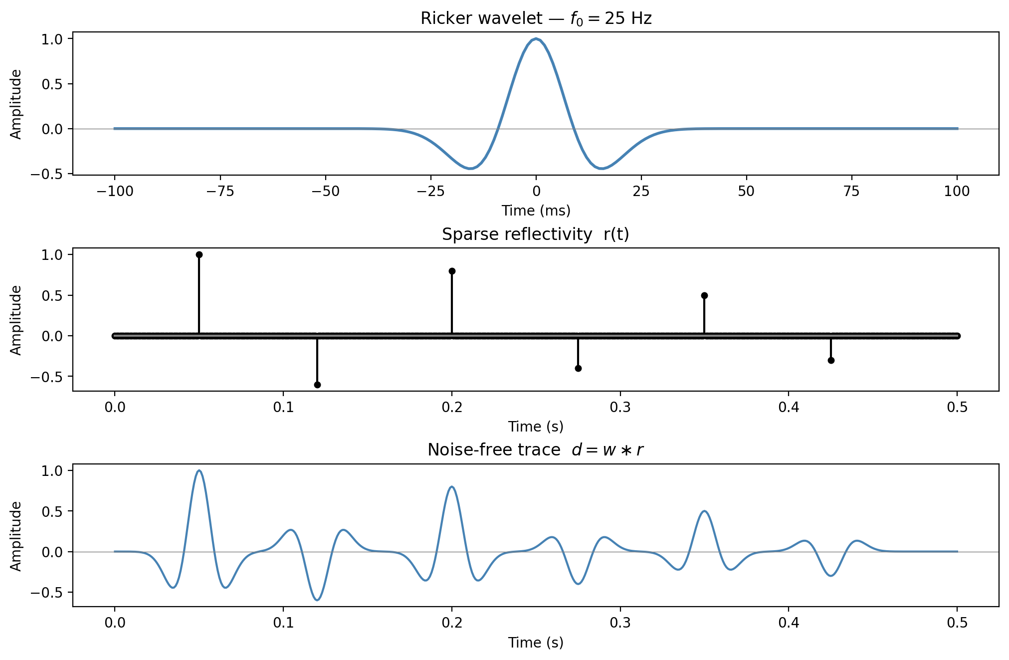
Example: reflectivity \(\ast\) Ricker wavelet
![]()
Each reflector produces a shifted, scaled copy of \(w(t)\); the seismogram \(d(t)\) is their superposition.
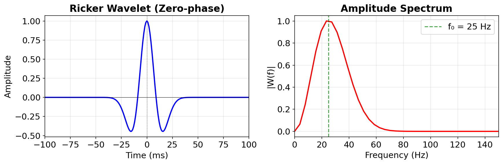
Ricker wavelet and its amplitude spectrum
![]()
The Ricker wavelet is band-limited — it has zero energy at DC \((f=0)\) and at high frequencies. Peak frequency \(f_0 = 25\) Hz.
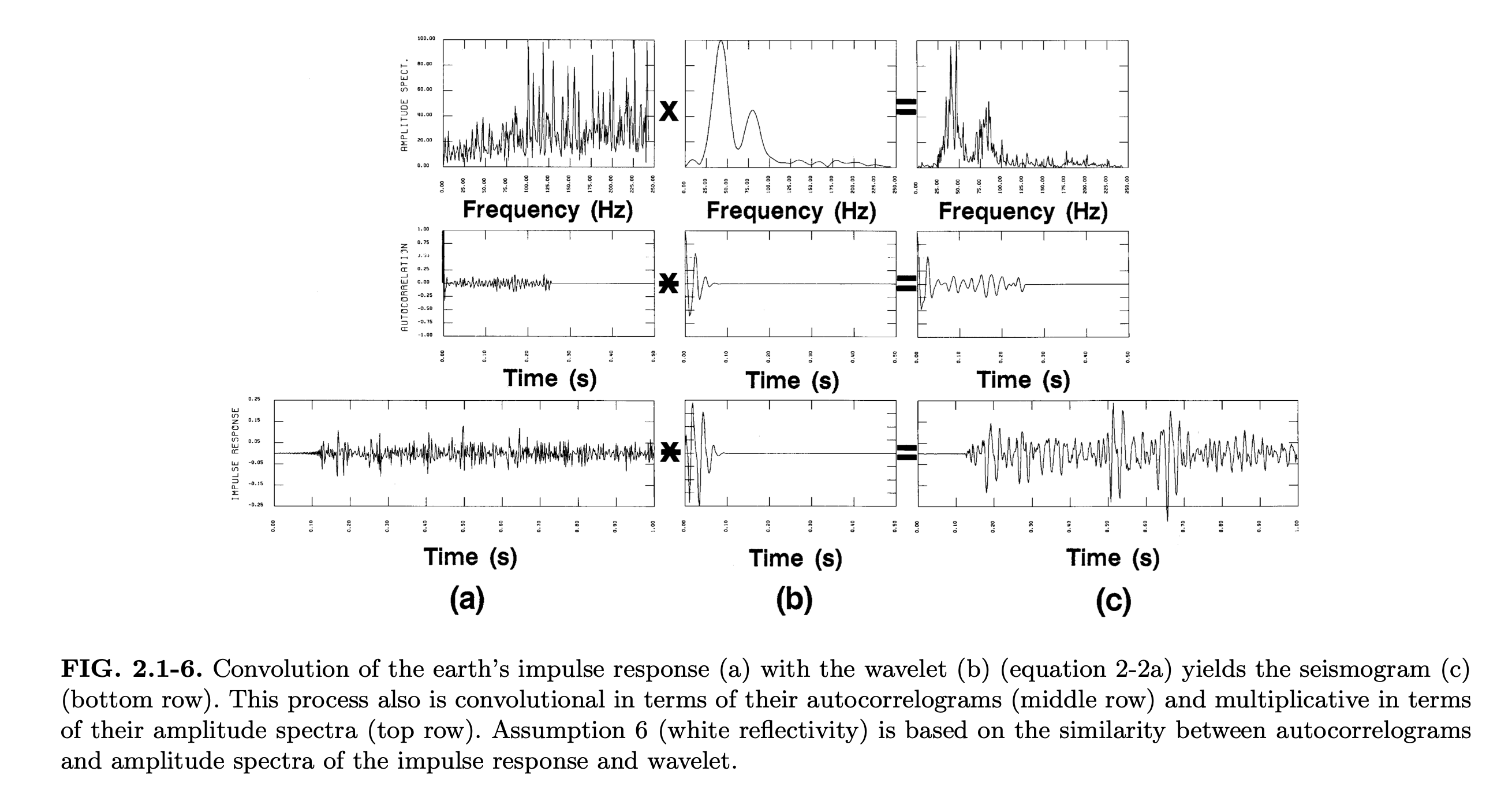
Convolution of the Earth impulse response
![]()
Convolution of earth’s impulse response (a) with wavelet (b) yields the seismogram (c). This is multiplicative in the amplitude spectra (top) and convolutional in the autocorrelations (middle). (Yilmaz 2001)
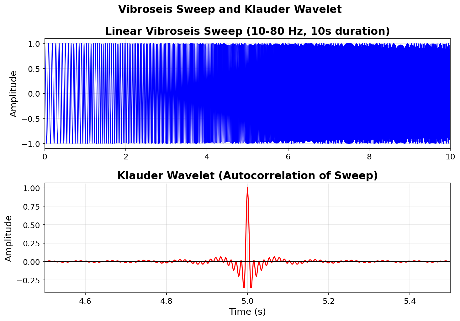
Vibroseis: sweep & Klauder wavelet
![]()
The vibroseis source emits a long frequency sweep. Cross-correlating the recorded data with the known sweep produces the Klauder wavelet — a compact, zero-phase pulse. (Sheriff and Geldart 1995)
Objective of deconvolution
Remove unwanted effects from the seismic signal to improve temporal resolution:
- Source/receiver characteristics — finite-bandwidth wavelet blurs the reflectivity
- Propagation effects — near-surface reverberations, ghosting
- Shallow water multiples — periodic repetitions from the water bottom
The aim is to recover a broadband, spike-like reflectivity \(r(t)\) from the recorded trace \(d(t)\).
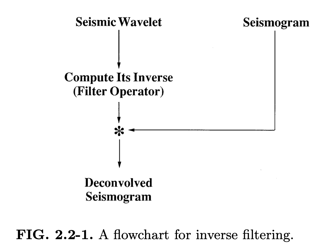
Deconvolution — the “inverse” problem
Goal: find \(r(t)\) from \(d(t) = w(t) \ast r(t) + n(t)\).
In the frequency domain the noise-free inverse is
\[
R(f) = \frac{D(f)}{W(f)}
\]
Equivalently, the inverse filter \(F(f) = 1/W(f)\) satisfies
\[
F(f)\, W(f) = 1 \quad \longleftrightarrow \quad f(t) \ast w(t) = \delta(t)
\]
The division-by-zero problem
Wherever \(W(f) \approx 0\) (spectral notches), the inverse \(1/W(f)\) blows up:
\[
\hat{R}(f) = R(f) + \frac{N(f)}{W(f)} \longrightarrow \infty
\]
Any small noise \(N(f)\) at those frequencies gets amplified enormously.
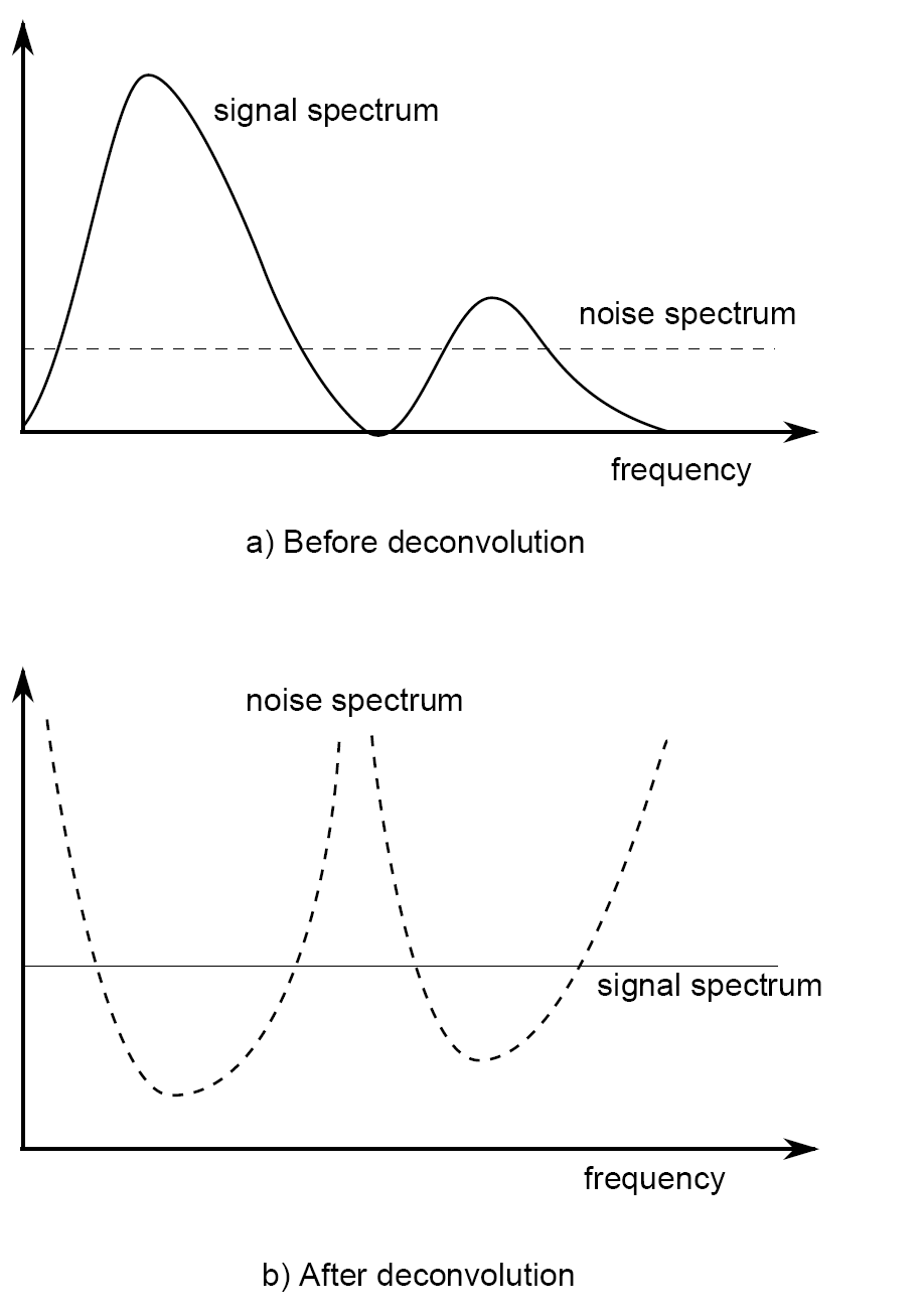
Deconvolution in the frequency domain
![]()
Adapted from Eric Verschuur
- Before deconvolution: signal spectrum dominates over noise.
- After naïve deconvolution: noise dominates at frequencies where \(|W(f)|\) is small.
Types of deconvolution
The term deconvolution is used for many different signal enhancement techniques:
| Spiking |
Sharpen wavelet \(\to\) spike \(\delta(t)\) |
Noise is Gaussian |
| Blind decon. |
Estimate source/receiver and earth response |
\(w(t)\) is minimum-phase, \(r(t)\) is white |
| Predictive |
Remove source/receiver ghosts and multiples |
Periodic structure in the data |
Main problem: the source/receiver responses and Earth response are both unknown. Given \(z = x \ast y\), what are \(x\) and \(y\)? This is the blind deconvolution problem.
Stabilized deconvolution — Wiener filter
Instead of \(1/W(f)\), use the Wiener filter (Wiener 1949):
\[
F(f) = \frac{W^*(f)}{|W(f)|^2 + \varepsilon}
\]
where \(\varepsilon > 0\) is the stabilization (damping) parameter that prevents division by zero.
Two regimes of the Wiener filter
\[
F(f) = \frac{W^*(f)}{|W(f)|^2 + \varepsilon}
\]
- when signal is strong: \(|W(f)|^2 \gg \varepsilon\)
\[F(f) \approx \frac{1}{W(f)} \qquad \Rightarrow \text{inverse filtering}\]
- when signal is weak: \(|W(f)|^2 \ll \varepsilon\)
\[F(f) \approx \frac{W^*(f)}{\varepsilon} \approx 0 \qquad \Rightarrow \text{suppress noisy frequencies}\]
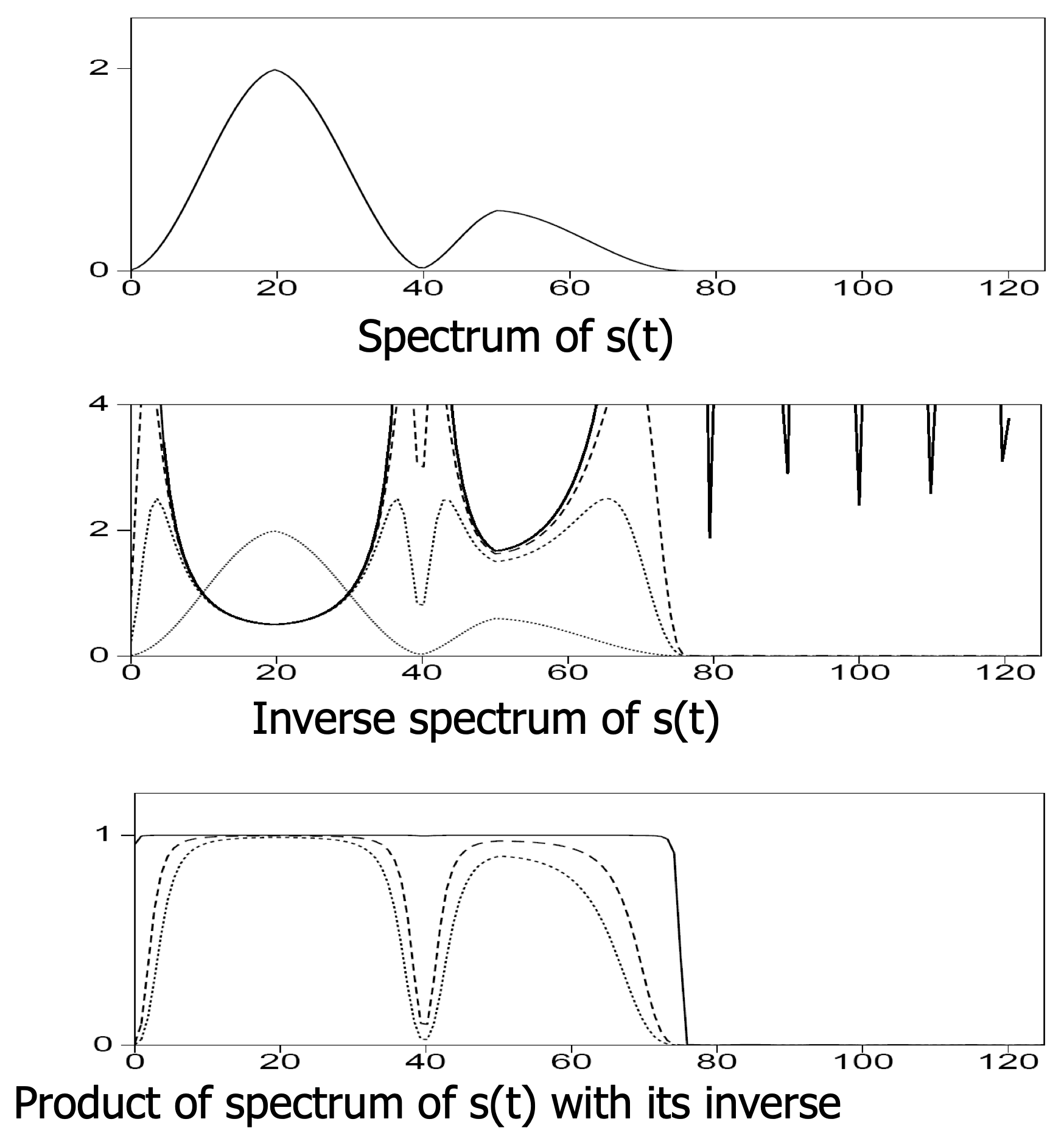
Stabilized noise-free
![]()
Adapted from Eric Verschuur
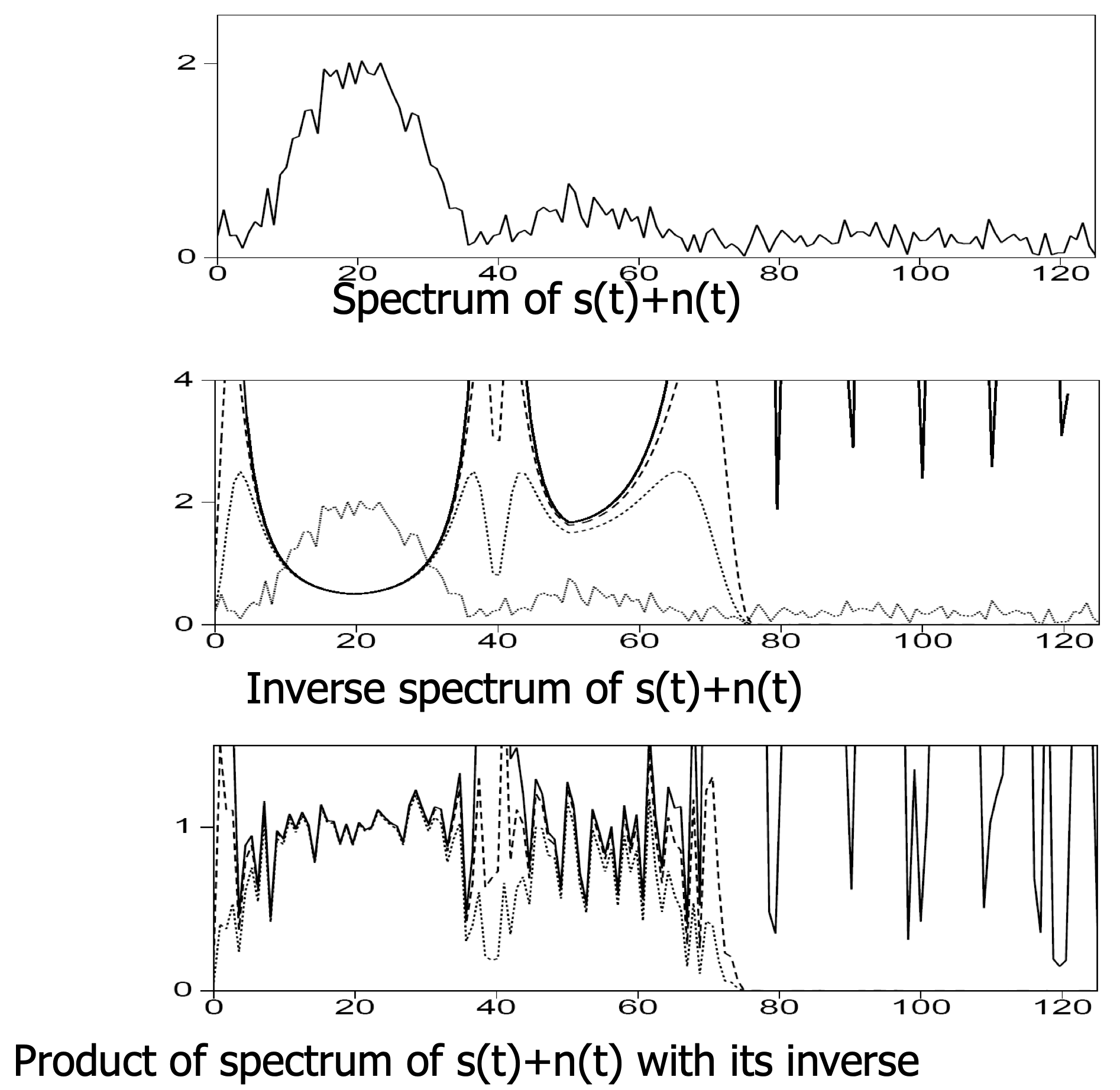
Stabilized noisy
![]()
Adapted from Eric Verschuur
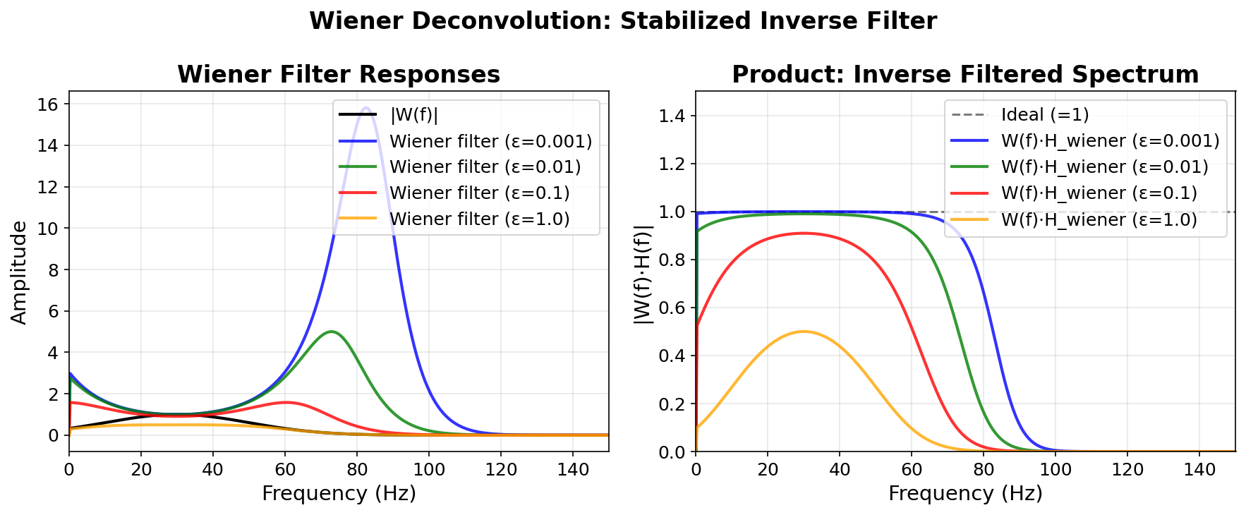
Wiener filter for different \(\varepsilon\)
![]()
Left: Wiener filter amplitude for \(\varepsilon \in \{0.001, 0.01, 0.1, 1.0\}\). Right: product \(W(f) \cdot F(f)\) — approaches \(1\) for small \(\varepsilon\), increasingly damped for large \(\varepsilon\).
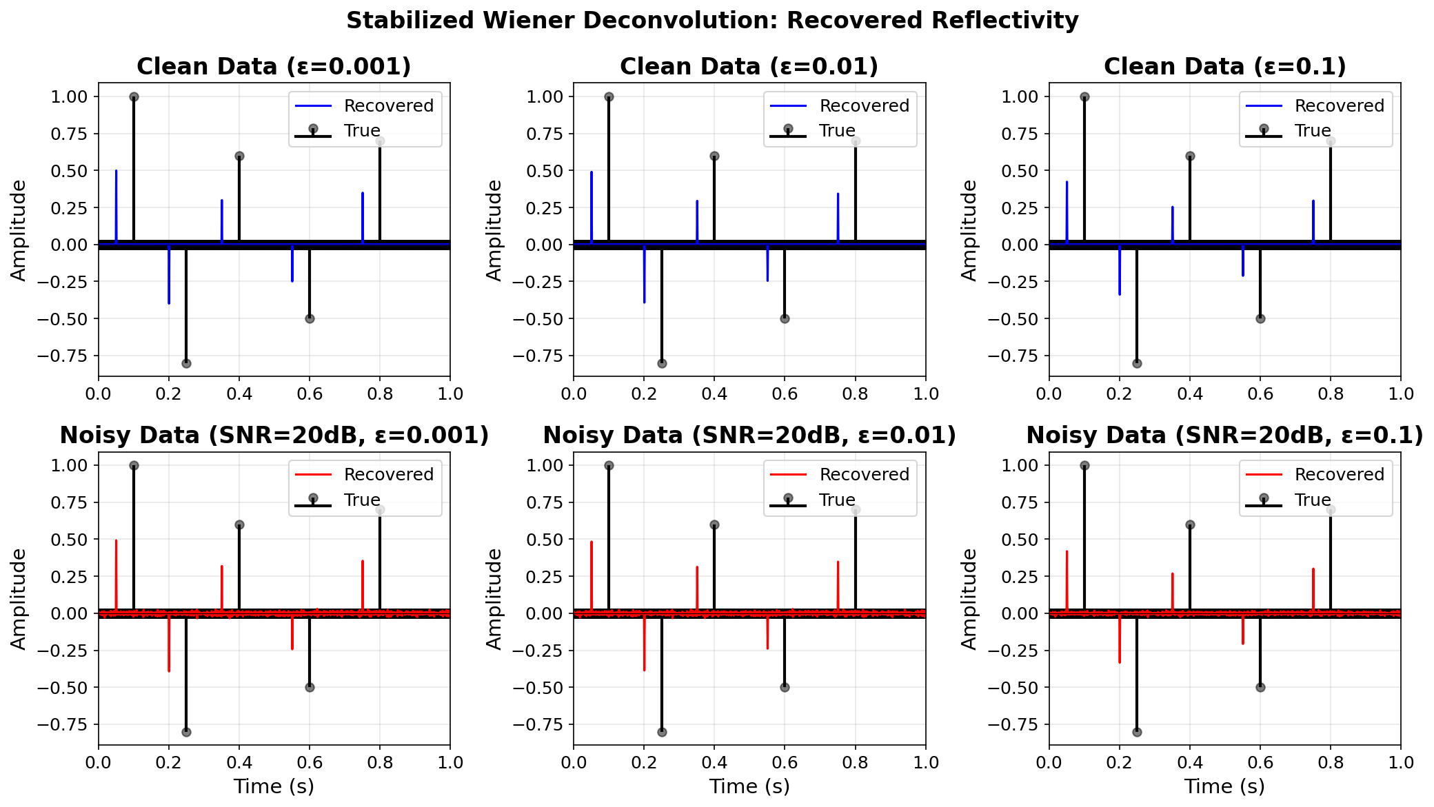
Stabilized deconvolution — results
![]()
Top: noise-free. Bottom: noisy (SNR = 20 dB). Small \(\varepsilon\) gives better resolution but amplifies noise — the classic resolution vs stability trade-off.
Setup: wavelet, reflectivity, and data
![]()
Ricker wavelet \(w(t)\) with \(f_0 = 25\) Hz convolved with a sparse reflectivity \(r(t)\) containing six isolated reflectors.
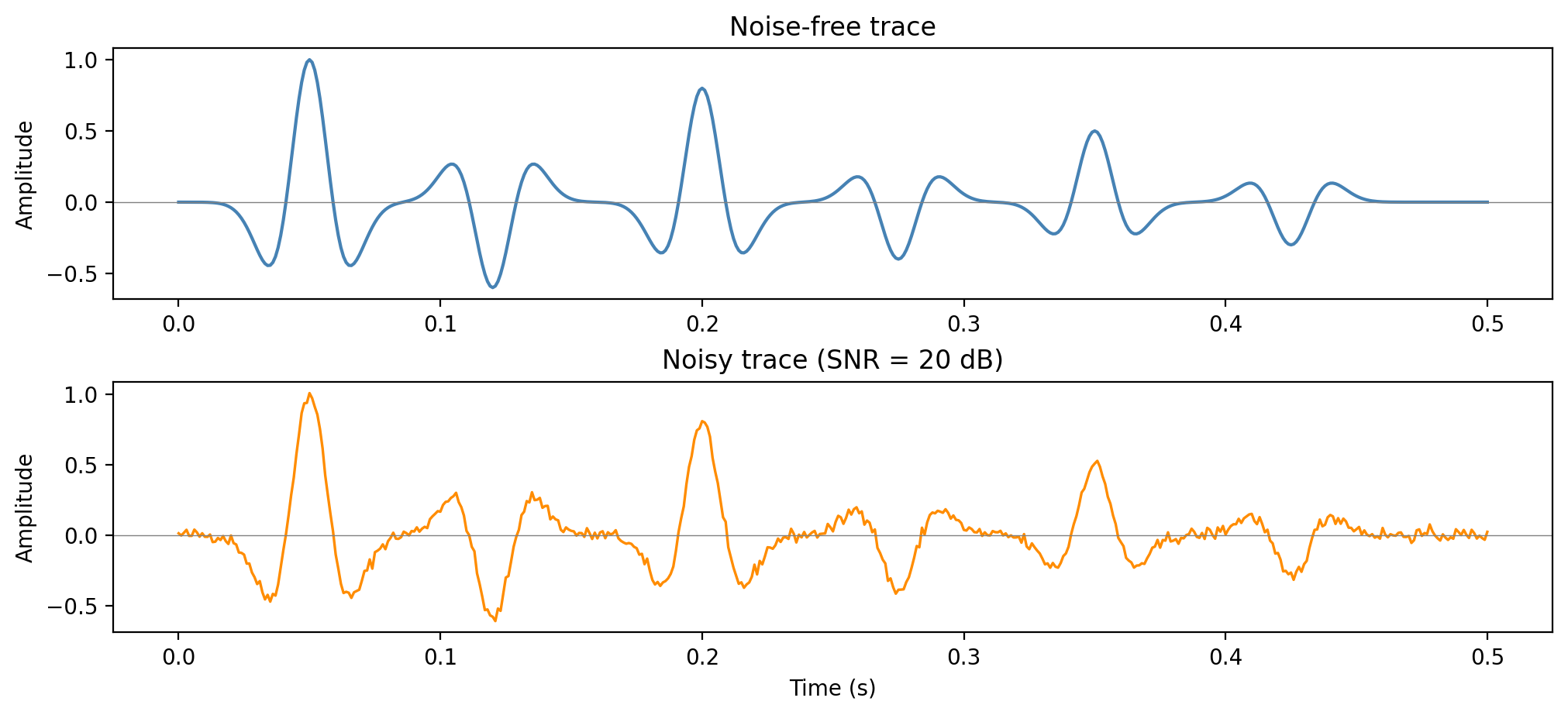
Noise-free vs noisy observed traces
![]()
Additive Gaussian noise at SNR = 20 dB. The noise is broadband — it contaminates all frequencies, including those where \(|W(f)| \approx 0\).
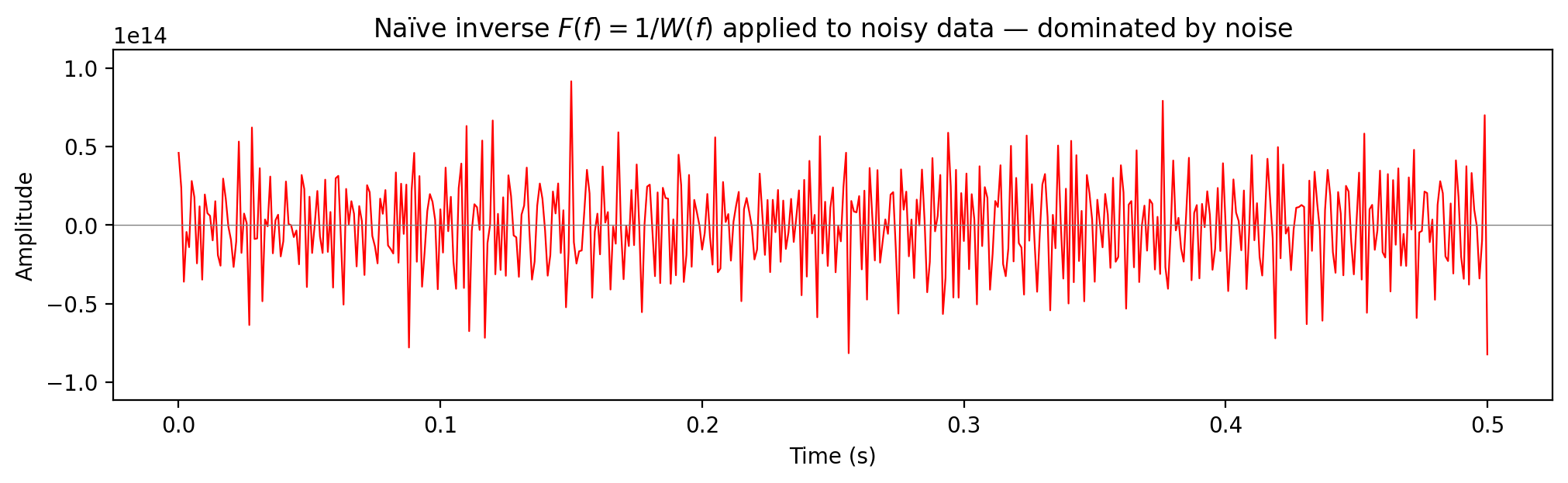
Naïve inverse: \(F(f) = 1/W(f)\)
![]()
Spectral division without stabilization. At spectral nulls of \(W(f)\) the noise is amplified without bound:
\[
\hat{R}(f) = R(f) + \frac{N(f)}{W(f)} \;\longrightarrow\; \infty
\]
The result is useless — completely dominated by amplified noise.
Wiener filter
The stabilized (Wiener) deconvolution filter:
\[
F_\varepsilon(f) = \frac{W^*(f)}{|W(f)|^2 + \varepsilon}
\]
Two regimes:
- \(|W(f)|^2 \gg \varepsilon\): \(\;F_\varepsilon(f) \approx 1/W(f)\) — inverse filtering
- \(|W(f)|^2 \ll \varepsilon\): \(\;F_\varepsilon(f) \approx W^*(f)/\varepsilon \approx 0\) — suppresses noisy frequencies
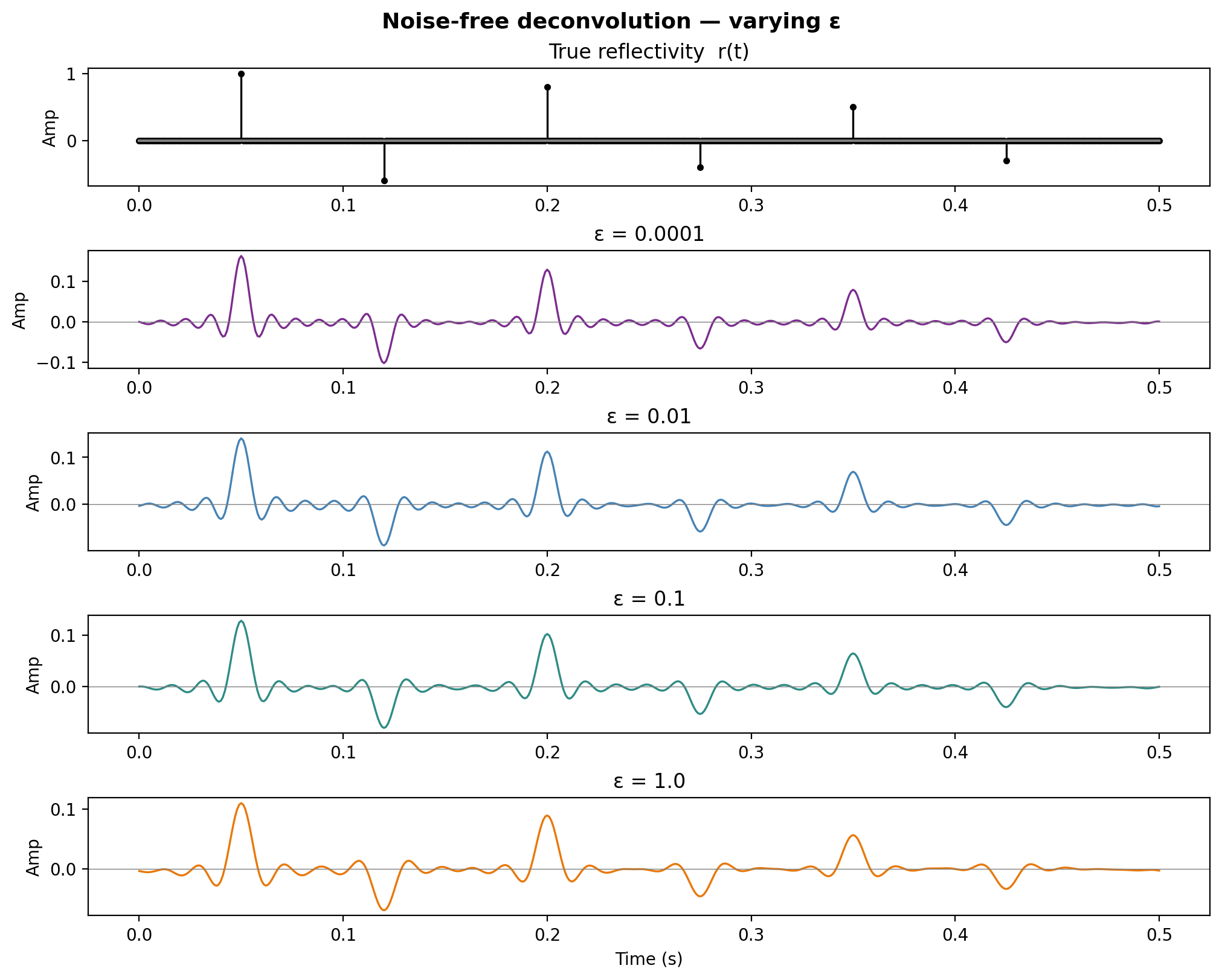
Noise-free deconvolution — varying \(\varepsilon\)
![]()
With no noise, small \(\varepsilon\) gives near-perfect recovery. As \(\varepsilon\) increases, the result becomes over-smoothed.
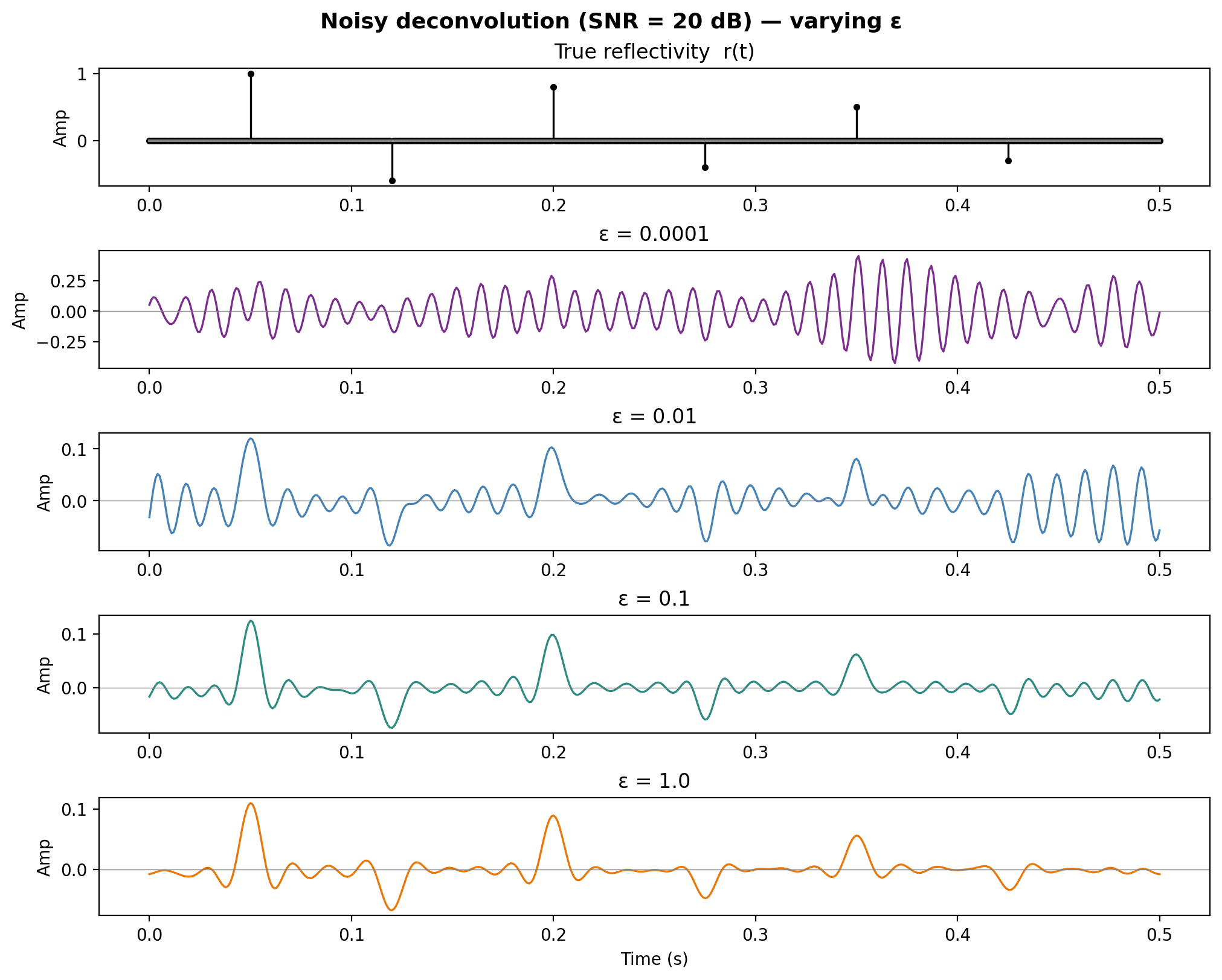
Noisy deconvolution — varying \(\varepsilon\)
![]()
With noise, small \(\varepsilon\) amplifies noise dramatically. Larger \(\varepsilon\) stabilizes the result at the cost of resolution.
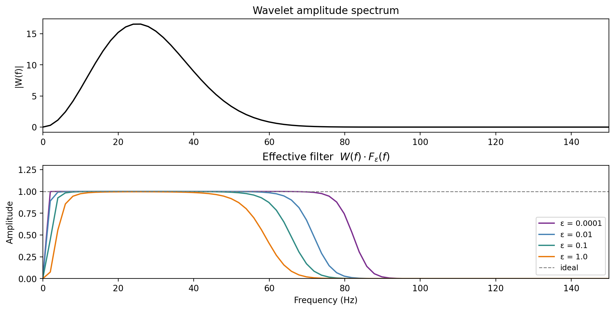
Frequency-domain view
![]()
Top: wavelet amplitude spectrum \(|W(f)|\). Bottom: effective resolution filter \(W(f) \cdot F_\varepsilon(f)\) — ideally unity across the signal band.
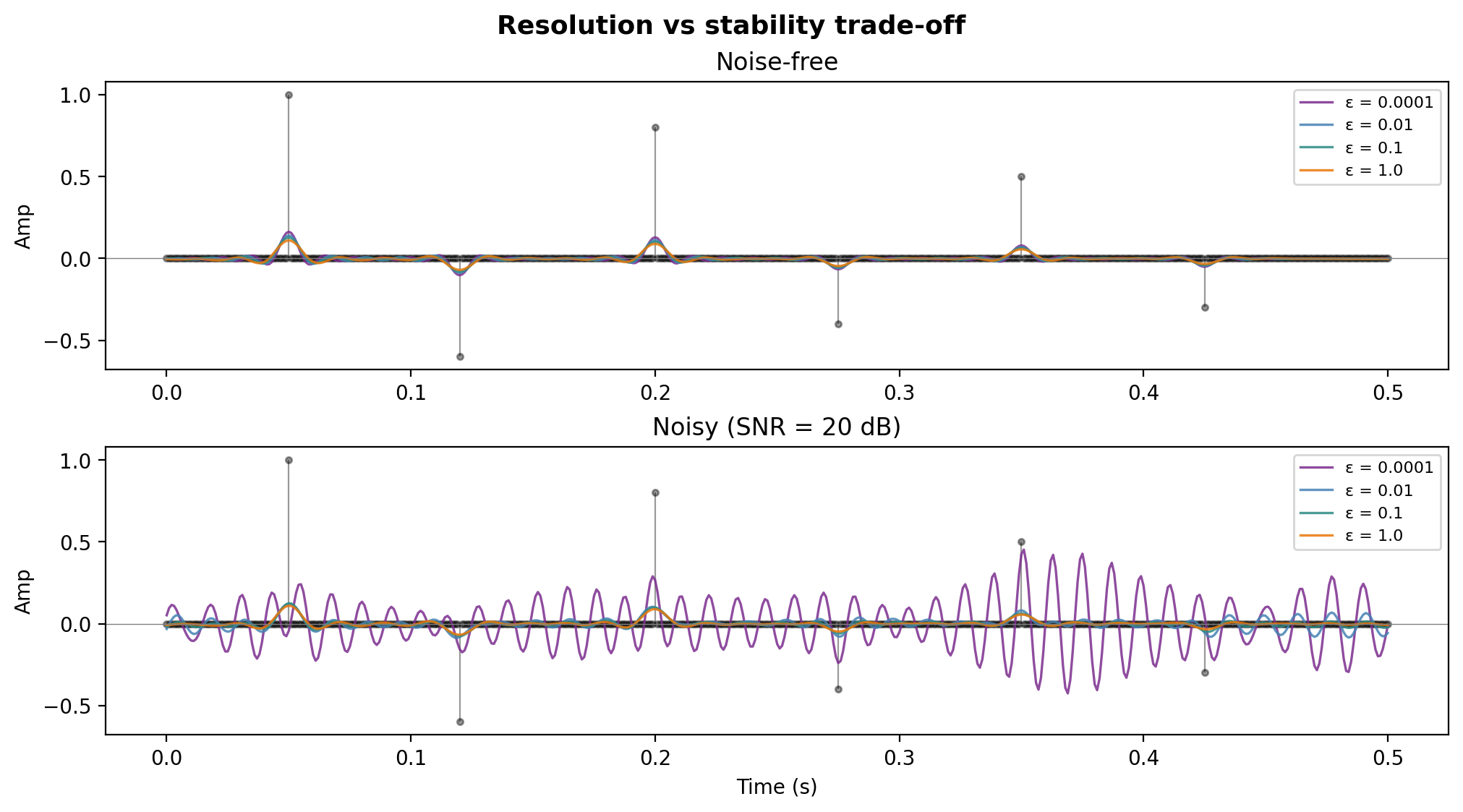
Resolution vs stability — the trade-off
![]()
All \(\varepsilon\) values overlaid with true \(r(t)\). Left: noise-free. Right: noisy. The optimal \(\varepsilon\) balances data misfit and noise amplification.
Summary
- Small \(\varepsilon\) — good resolution but amplifies noise
- Large \(\varepsilon\) — stable but over-smoothed (loss of resolution)
- The optimal \(\varepsilon\) balances data misfit and noise amplification
- In practice \(\varepsilon\) is chosen as a fraction of \(\max|W(f)|^2\) or estimated from the noise level—i.e., \(\varepsilon=0.05 \max|W(f)|^2\)
Time-domain: least-squares formulation
In the time domain, deconvolution becomes a least-squares problem. Given data vector \(\mathbf{d}\) and convolution matrix \(\mathbf{W}\):
\[
\min_{\mathbf{r}} \|\mathbf{d} - \mathbf{W}\mathbf{r}\|_2^2
\]
The normal equations that solve this objective give
\[
\mathbf{W}^T \mathbf{W}\, {\mathbf{r}} = \mathbf{W}^T \mathbf{d}
\]
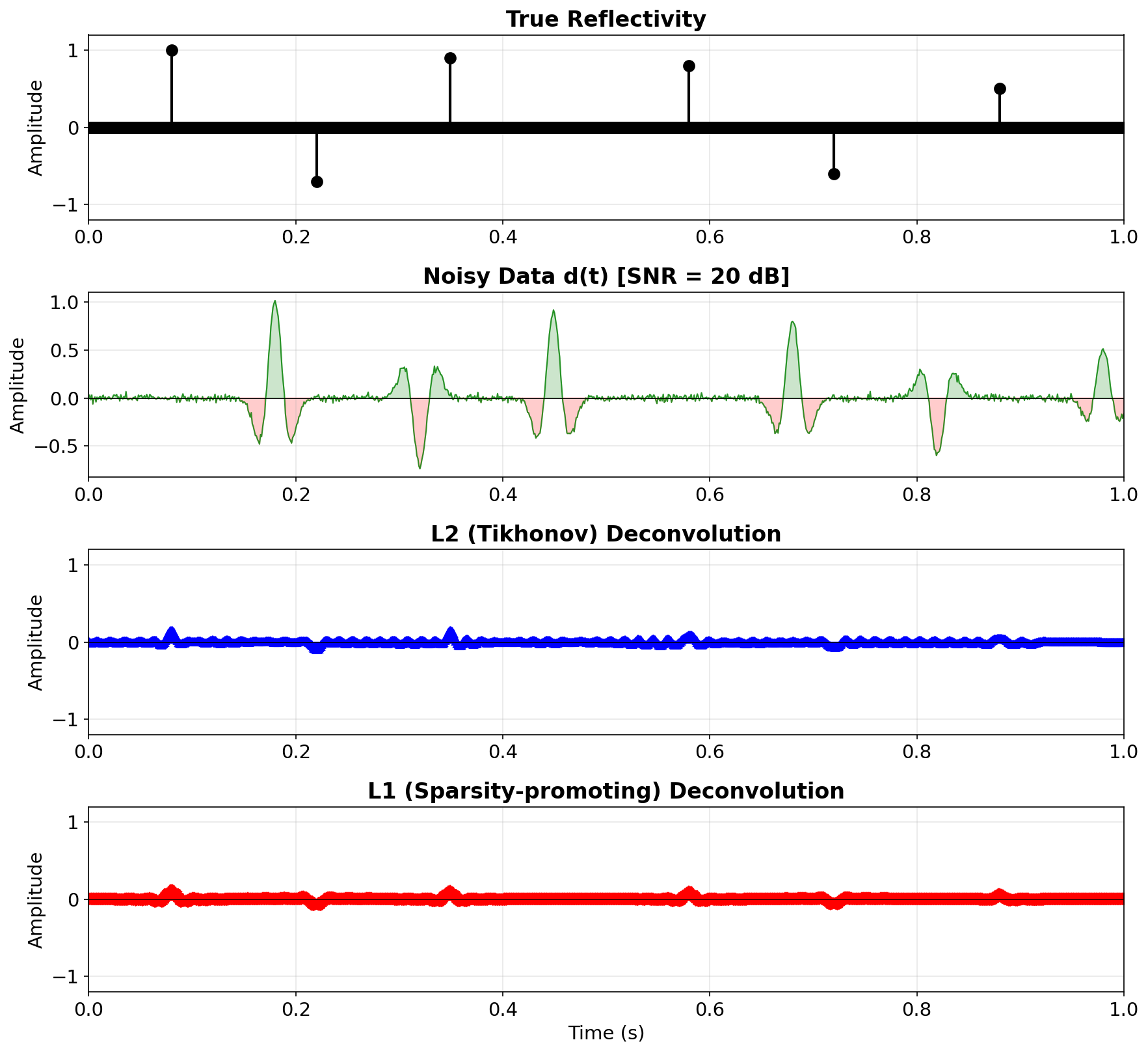
Tikhonov regularization
Adding an \(\ell_2\)-penalty on \(\mathbf{r}\) yields the damped (Tikhonov regularized) problem:
\[
\min_{\mathbf{r}} \|\mathbf{d} - \mathbf{W}\mathbf{r}\|_2^2 + \varepsilon \|\mathbf{r}\|_2^2
\]
with closed-form solution
\[
\tilde{\mathbf{r}} = (\mathbf{W}^T\mathbf{W} + \varepsilon \mathbf{I})^{-1}\, \mathbf{W}^T \mathbf{d}
\]
This is exactly the Wiener filter in the time domain. The Fourier-domain Wiener filter and Tikhonov regularization are equivalent for stationary convolution.
Time-domain Wiener filter design
We want a approximate short deconvolution filter \(f(t)\) that replaces the original source wavelet \(w(t)\) by a desired wavelet \(v(t)\):
\[f(t)\ast w(t)=v(t)\]
Write objective
\[\min_{\mathbf{f}\in F} \|\mathbf{v} - \mathbf{f}\ast\mathbf{w}\|_2^2 \]
with \(F\) set of short wavelets, which is solved by
\[f\ast r_{ww} = r_{vw}\]
where
the auto-correlation \(r_{ww}[k] = \sum_n w[n]\, w[n+k]\)
the cross-correlation \(r_{dw}[k] = \sum_n d[n]\, w[n+k]\)
Toeplitz structure of normal equations
\[
\begin{bmatrix} r_{ww}[0] & r_{ww}[1] & \cdots & r_{ww}[N{-}1] \\ r_{ww}[1] & r_{ww}[0] & \cdots & r_{ww}[N{-}2] \\ \vdots & & \ddots & \vdots \\ r_{ww}[N{-}1] & r_{ww}[N{-}2] & \cdots & r_{ww}[0] \end{bmatrix} \begin{bmatrix}f[0]\\ f[1] \\ \vdots \\ f[N]\end{bmatrix} = \begin{bmatrix} r_{vw}[0] \\ r_{vw}[1] \\ \vdots \\ r_{vw}[N] \end{bmatrix}
\]
This symmetric Toeplitz system can be solved in \(O(N^2)\) via the Levinson recursion (Levinson 1947), rather than \(O(N^3)\) for general systems.
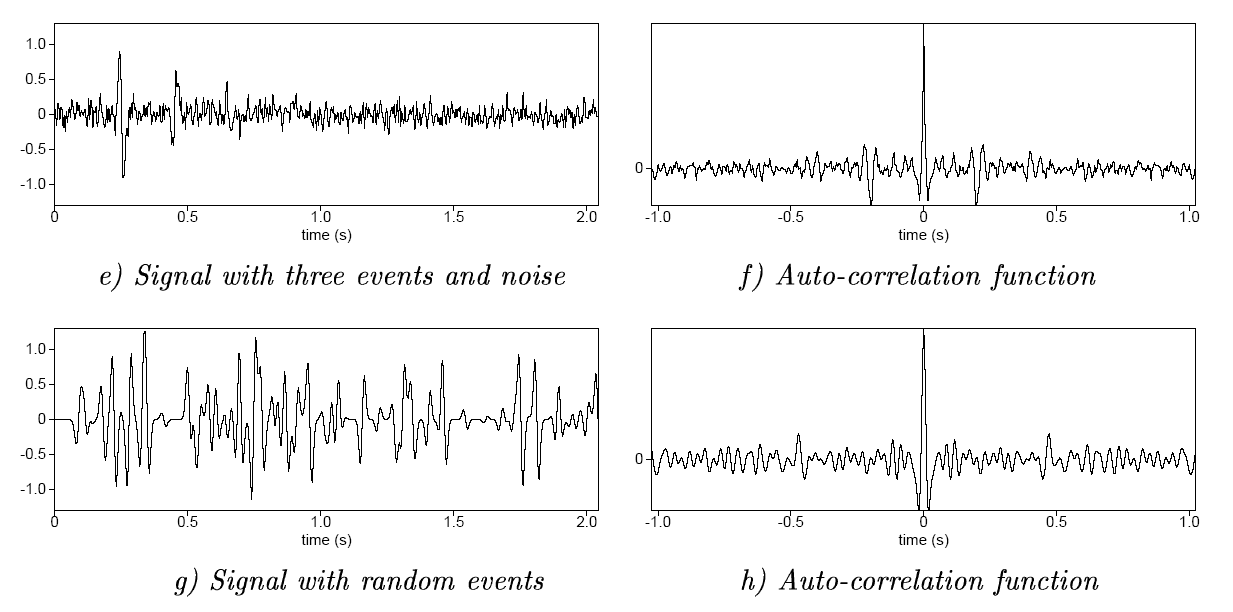
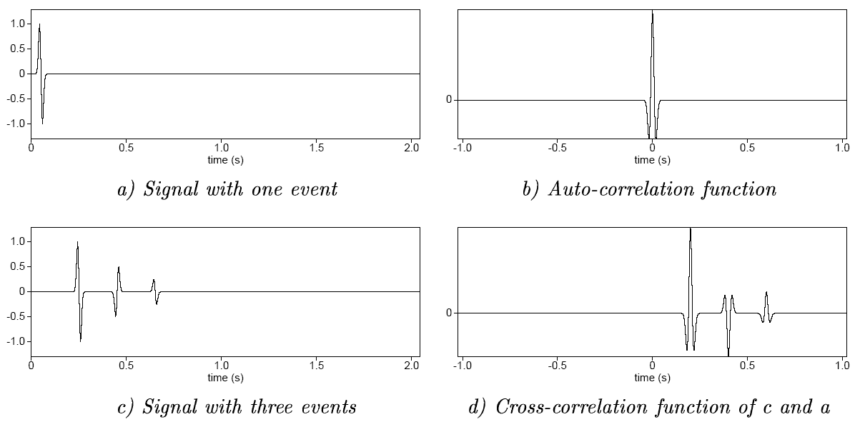
Auto- and cross-correlation examples
![]()
Yilmaz (2001)
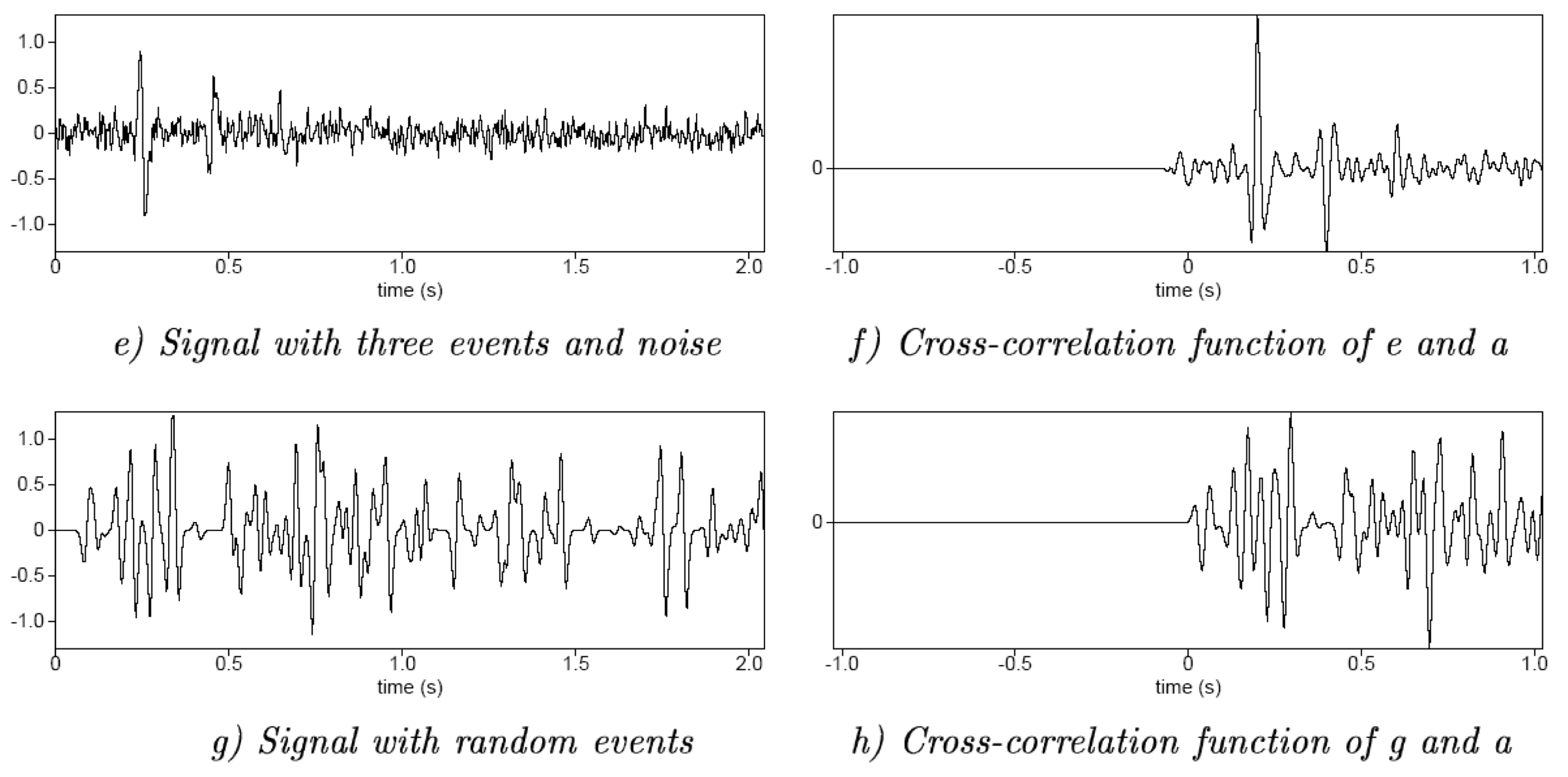
Auto- and cross-correlation examples
![]()
Yilmaz (2001)
Auto- and cross-correlation examples
![]()
Yilmaz (2001)
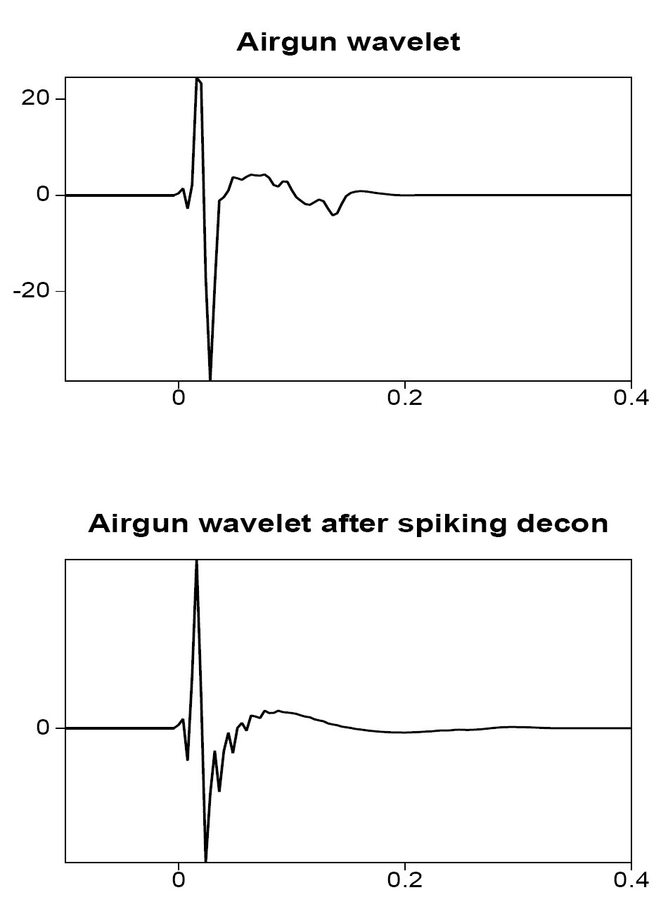
Example: spiking deconvolution — wavelet
![]()
Airgun wavelet (top) and result after spiking deconvolution (bottom) — the wavelet is compressed toward a spike \(\delta(t)\).
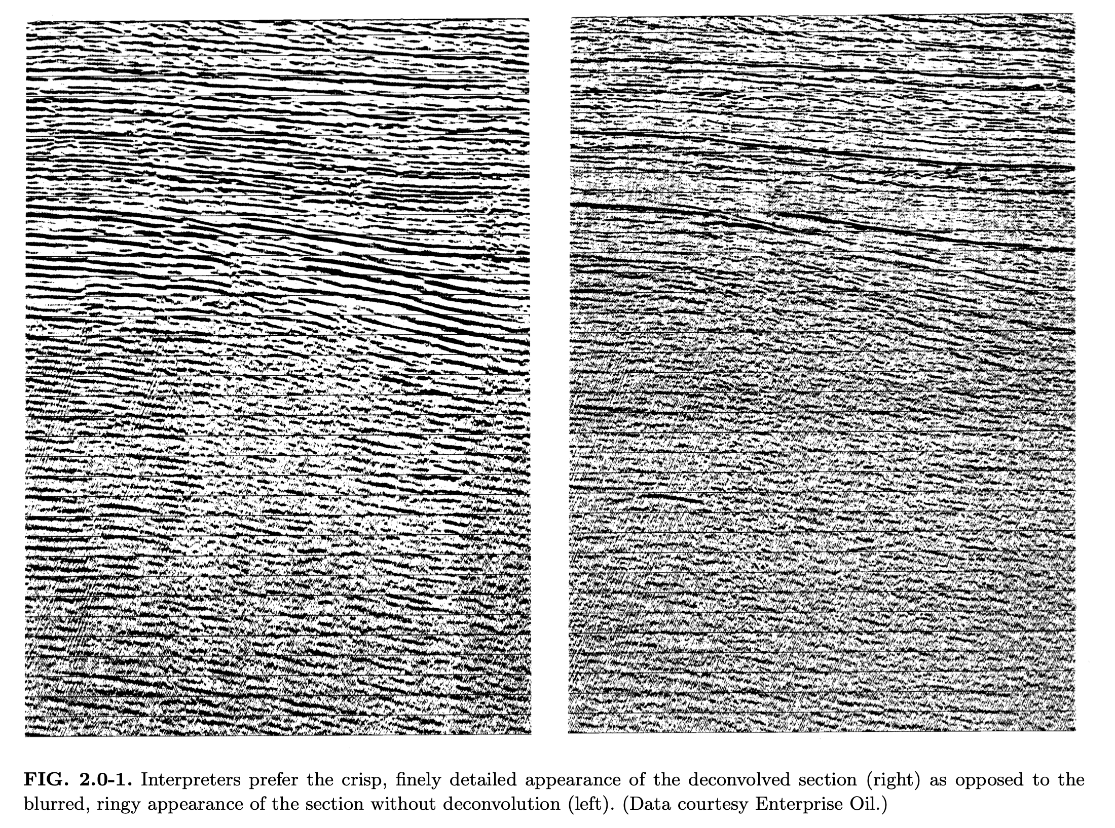
Spiking deconvolution — shot gather
![]()
Shot gather before (left) and after (right) spiking deconvolution — reflectors become sharper and more interpretable.
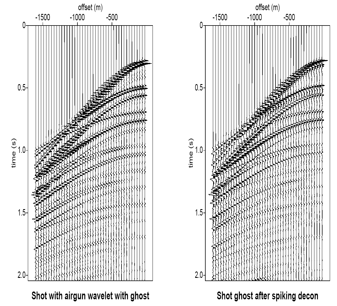
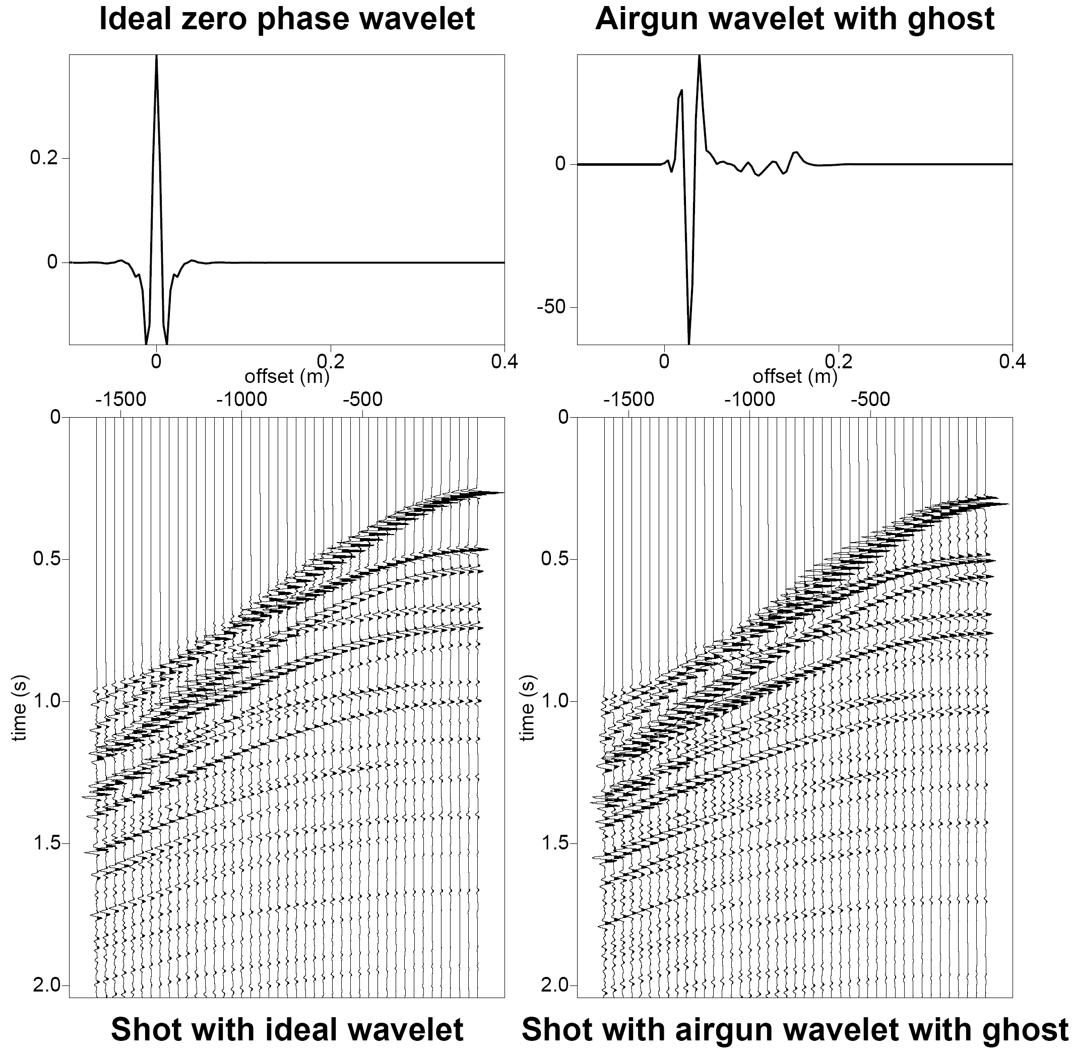
Modeling example: ideal vs airgun wavelet
![]()
Left: ideal zero-phase wavelet and corresponding shot gather. Right: realistic airgun wavelet with ghost — note the longer, ringy waveform that obscures reflector boundaries.
Part III — Predictive deconvolution
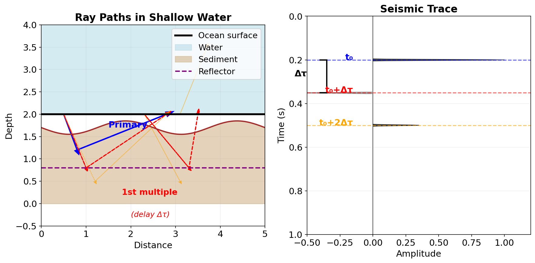
Predictive deconvolution — motivation
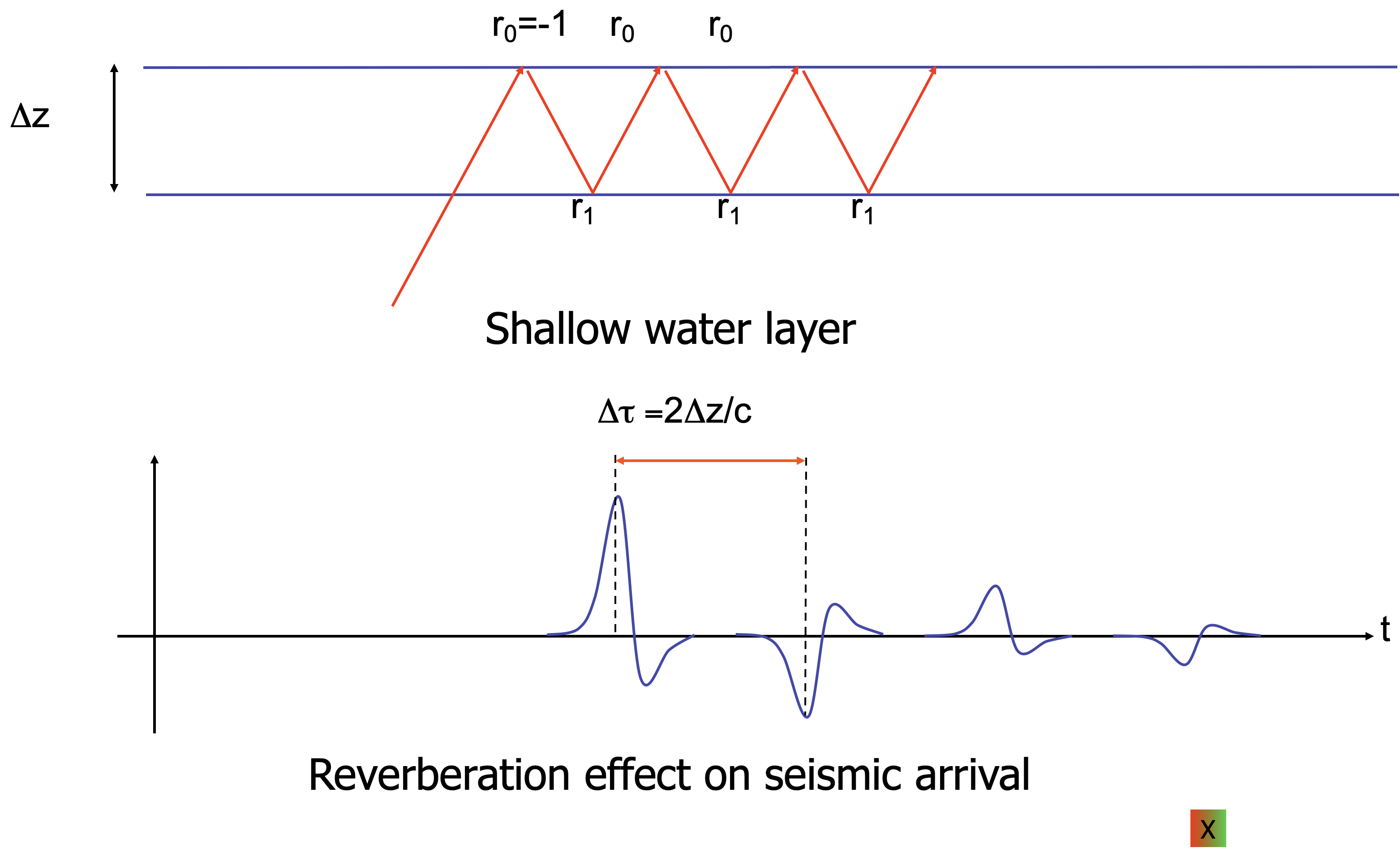
Predictive deconvolution aims at removing a repetitive character from the seismic measurements, not the source signal itself. This can be used in the following situations:
- the source signal itself has a repetitive character, e.g. the airgun bubble effect
- certain layer generates strong reverberations, e.g. a shallow water layer
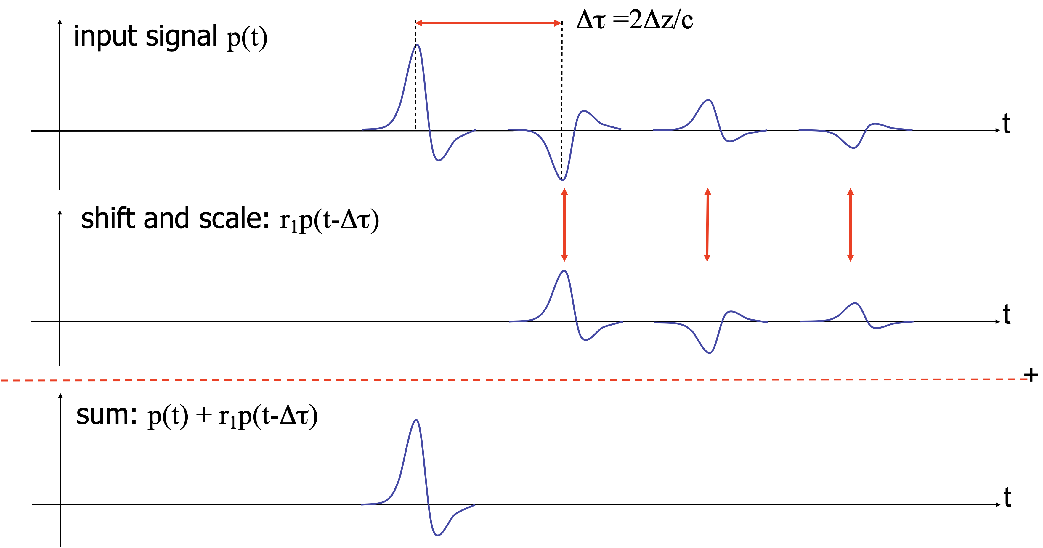
In this situation, the seismic trace with reverberations can be written as a geometric series:
\[
d(t) = p(t) + r_1\, p(t - \Delta\tau) + r_1^2\, p(t - 2\Delta\tau) + \cdots
\]
where \(p(t)\) is the primary signal, \(\Delta\tau\) is the two-way travel time in the water layer, and \(r_1\) is the water-bottom reflection coefficient.
Idea: if we can predict the signal \(\Delta\tau\) into the future, we can subtract the predictable (periodic) part. (Robinson 1967)
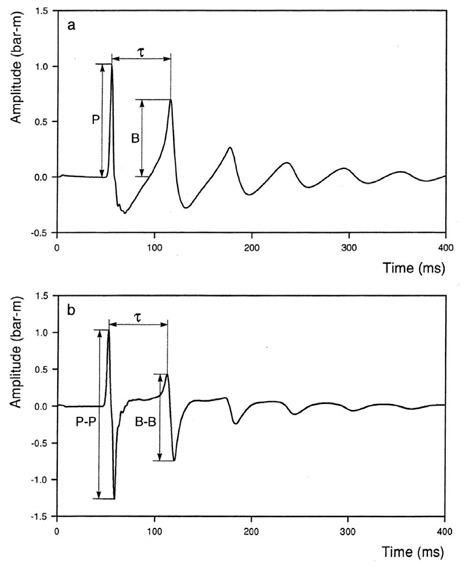
Examples periodic
![]()
adapted from Eric Verschuur
Ocean bottom multiples
![]()
adapted from Eric Verschuur
Ocean bottom multiple removal
![]()
adapted from Eric Verschuur
Predictive deconvolution — filter design
The prediction-error filter has the form
\[
f_{\text{pred}}(t) = \delta(t) - a(t - \Delta\tau)
\]
where \(a(t)\) is a prediction filter that estimates \(d(t)\) from \(d(t - \Delta\tau)\).
![]()
Left: ideal filter. Right: practical filter designed from data.
Predictive decon — least-squares objective
The prediction filter \(\mathbf{a}\) is found by minimizing
\[
\min_{\mathbf{a}} \sum_n \left| d[n] - \sum_k a[k]\, d[n - \Delta - k] \right|^2
\]
where \(\Delta\) is the prediction distance (in samples). The normal equations are
\[
\mathbf{R}_{dd}\, \hat{\mathbf{a}} = \mathbf{r}_{dd}[\Delta]
\]
Spiking deconvolution is the special case \(\Delta = 1\) (predict one sample ahead). Multiple removal uses \(\Delta = \Delta\tau / \Delta t\) (predict one multiple period ahead).
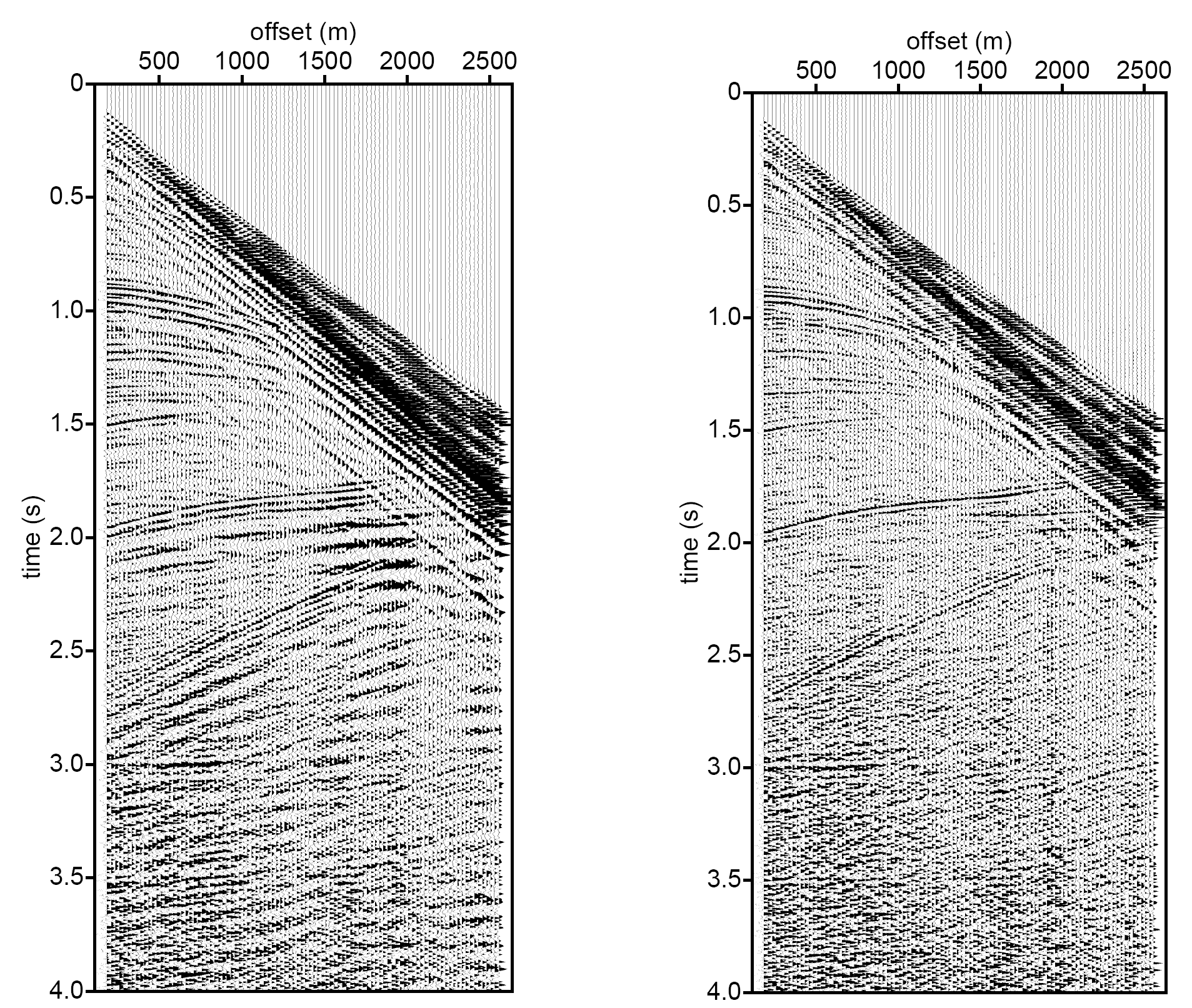
Example: predictive deconvolution — shot record
![]()
Adapted from Eric Verschuur
Original shot record with shallow-water multiples (left) vs after predictive deconvolution (right). The reverberations are strongly attenuated.
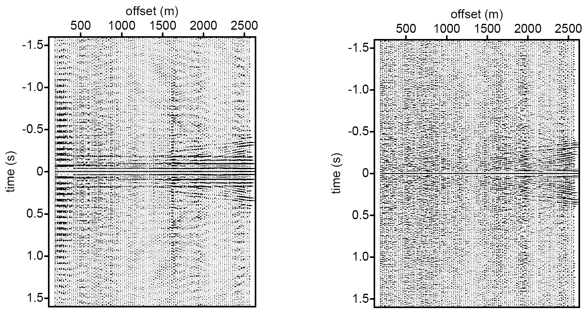
Predictive decon — autocorrelation check
![]()
Autocorrelation of input (left) shows periodic structure from multiples. After predictive deconvolution (right) the periodicity is removed — the autocorrelation approaches a spike.