Flow Matching & Score-Based Diffusion
Digital Twins for Physical Systems
2026-03-04


Flow Matching & Score-Based Diffusion
a tutorial
Felix J. Herrmann
School of Computational Science and Engineering — Georgia Institute of Technology
Slides build on Holderrieth and Erives (2025) — Course website
The Flow: Warping Space
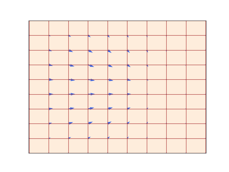
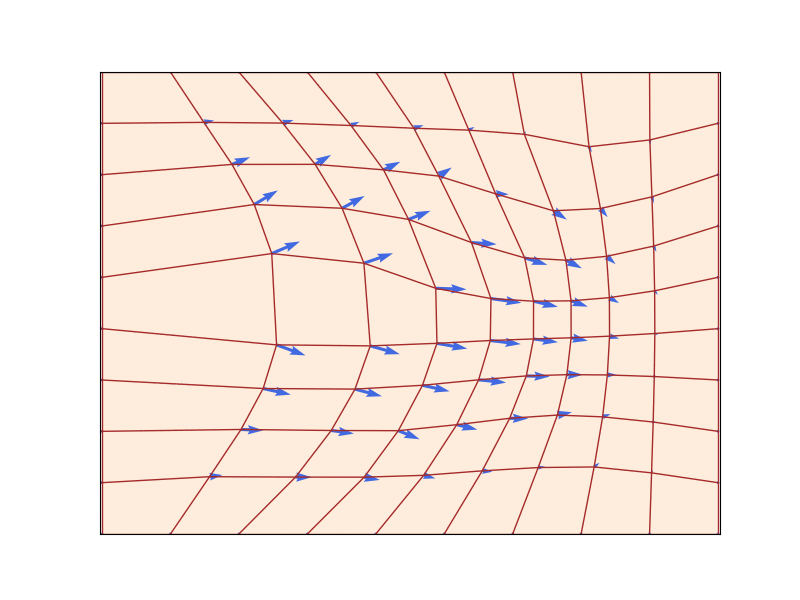
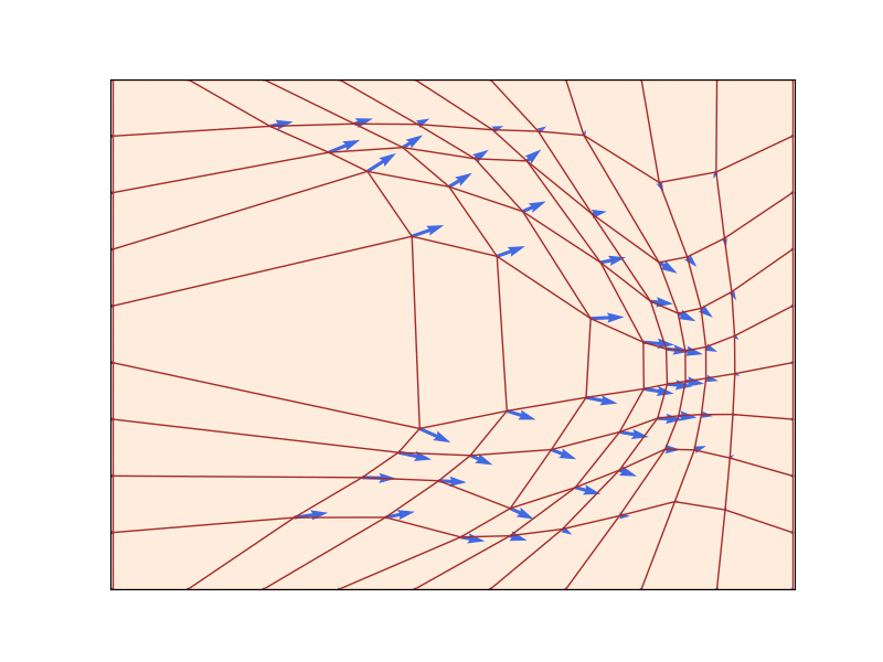
A flow \(\psi_t: \mathbb{R}^d \to \mathbb{R}^d\) (red grid) defined by a velocity field \(u_t\) (blue arrows) that prescribes instantaneous movements (\(d=2\)). A flow is a diffeomorphism that “warps” space. Figure from Lipman et al. (2024).
Existence & uniqueness: If \(u_t\) is continuously differentiable with bounded derivative, the ODE has a unique flow \(\psi_t\) that is a diffeomorphism (Perko 2013).
Ornstein-Uhlenbeck Processes
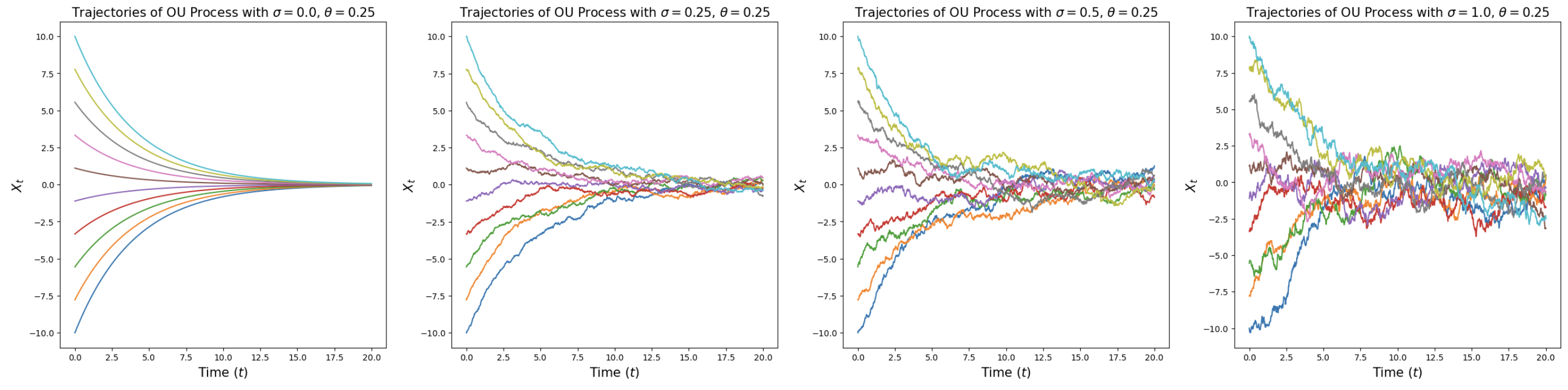
Ornstein-Uhlenbeck processes \(\mathrm{d}X_t = -\theta X_t\,\mathrm{d}t + \sigma\,\mathrm{d}W_t\) for \(\theta = 0.25\) and various \(\sigma\). For \(\sigma = 0\): deterministic flow converging to origin. For \(\sigma > 0\): random paths converging to \(\mathcal{N}(0, \sigma^2/(2\theta))\). From Holderrieth and Erives (2025).
The Training Problem
We need to train \(u_t^\theta\) by minimizing a loss:
\[\mathcal{L}(\theta) = \|u_t^\theta(x) - \underbrace{u_t^\text{target}(x)}_{\text{training target}}\|^2\]
Two-step approach:
- Find the training target \(u_t^\text{target}\): a vector field whose ODE/SDE converts \(p_\text{init}\) into \(p_\text{data}\)
- Train \(u_t^\theta\) to approximate \(u_t^\text{target}\)
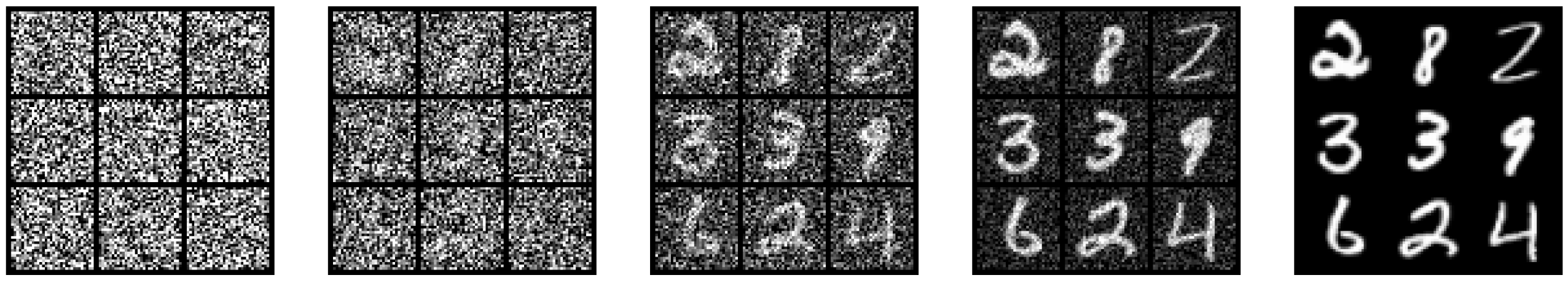
Conditional Probability Path
Variational diffusion model: forward noising process. From Kreis et al. (2022).
A conditional probability path \(p_t(x \mid z)\) is a family of distributions over \(\mathbb{R}^d\) such that:
\[p_0(\cdot \mid z) = p_\text{init}, \qquad p_1(\cdot \mid z) = \delta_z \qquad \forall z \in \mathbb{R}^d\]
It gradually converts a single data point \(z\) into \(p_\text{init}\).
Gaussian Conditional Probability Path
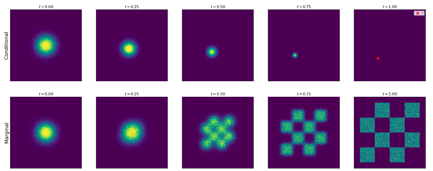
Conditional (top) vs marginal (bottom) probability path for Gaussian path with \(\alpha_t = t, \beta_t = 1-t\). From Holderrieth and Erives (2025).
\[p_t(\cdot \mid z) = \mathcal{N}(\alpha_t z, \beta_t^2 I_d)\]
where \(\alpha_t, \beta_t\) are noise schedulers: monotonic with \(\alpha_0 = \beta_1 = 0\), \(\alpha_1 = \beta_0 = 1\).
Sampling from the marginal path: \(\;z \sim p_\text{data},\; \epsilon \sim \mathcal{N}(0, I_d) \;\Rightarrow\; x = \alpha_t z + \beta_t \epsilon \sim p_t\)
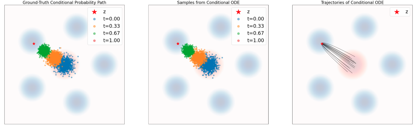
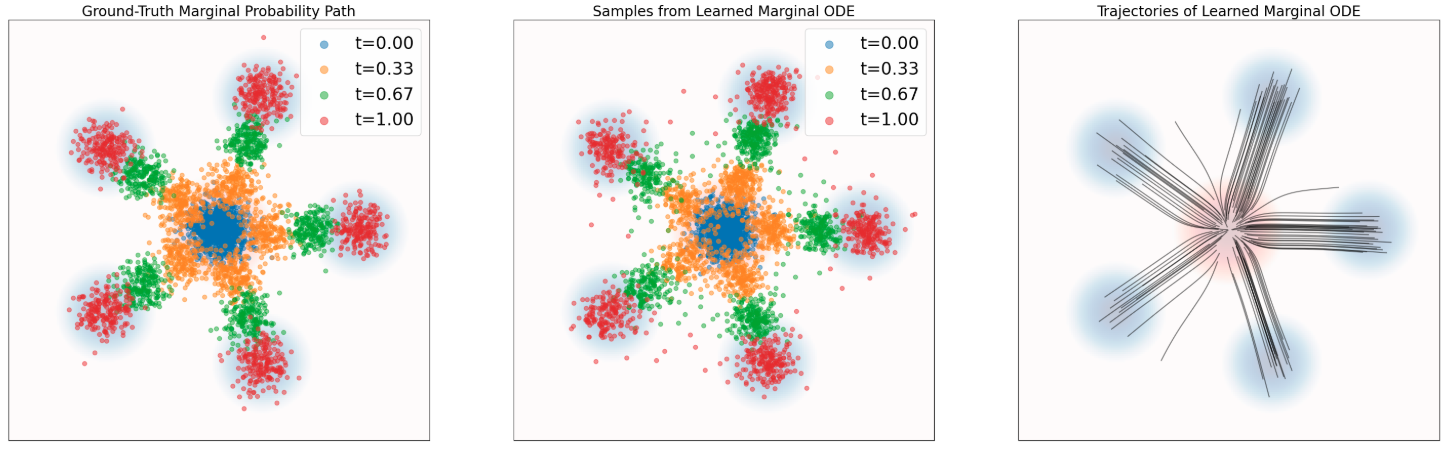
Conditional vs Marginal ODE
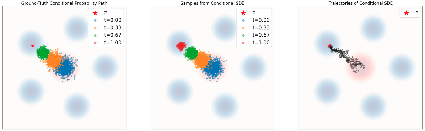
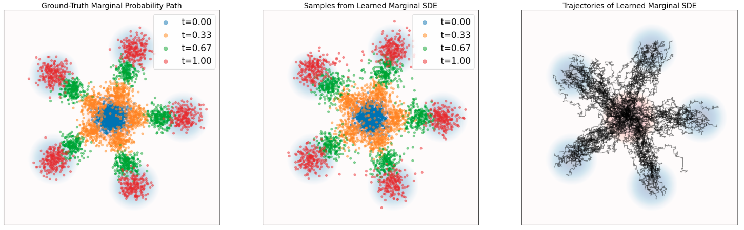
SDE Extension Trick
Score-Based Sampling: Langevin Dynamics
Langevin dynamics is a special case where \(p_t = p\) is static and \(u_t^\text{target} = 0\):
\[\mathrm{d}X_t = \frac{\sigma_t^2}{2}\nabla \log p(X_t)\,\mathrm{d}t + \sigma_t\,\mathrm{d}W_t\]
The distribution \(p\) is a stationary distribution: \(X_0 \sim p \;\Rightarrow\; X_t \sim p\;\;(t \geq 0)\).
Under mild conditions, \(X_t \to p\) regardless of initialization.
This is the basis of molecular dynamics simulations and MCMC methods.
Langevin Dynamics: Convergence
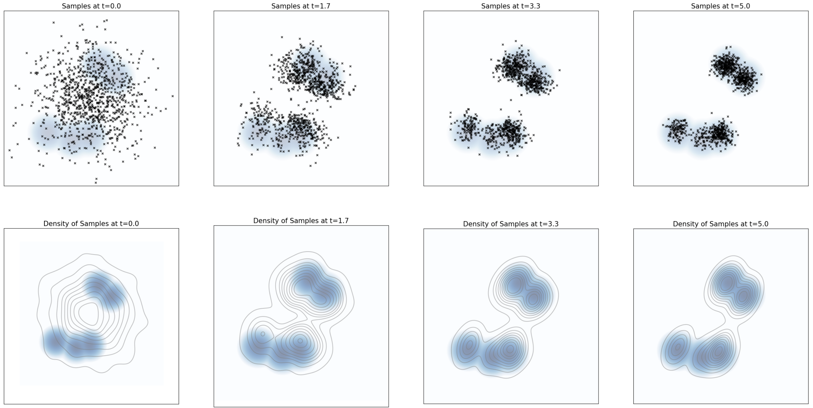
Particles evolving under Langevin dynamics with \(p(x)\) taken to be a Gaussian mixture with 5 modes. The distribution of samples converges to the equilibrium distribution \(p\) (blue background). From Holderrieth and Erives (2025).
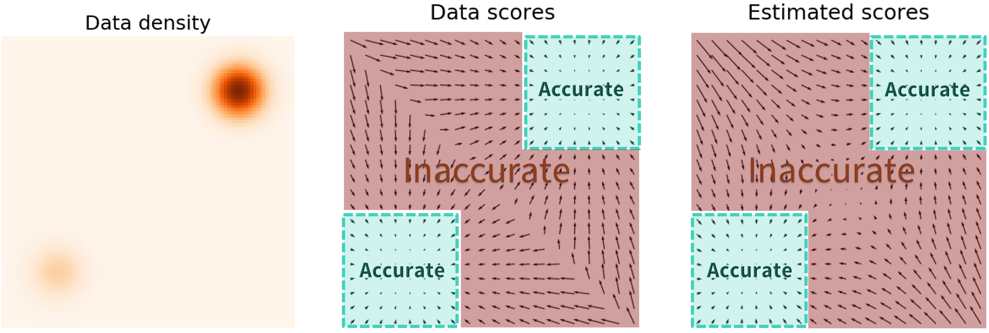
Score Estimation: Pitfalls
Estimating the score \(\nabla \log p(x)\) in low-density regions is inaccurate because few data points are available there.
Solution: Perturb data with multiple noise levels to fill in low-density regions (Song and Ermon 2019).
Annealed Langevin Dynamics
Train score networks at multiple noise levels and use annealed Langevin dynamics: start with high noise, gradually decrease.
This gives accurate score estimates throughout the space and enables high-quality sampling.
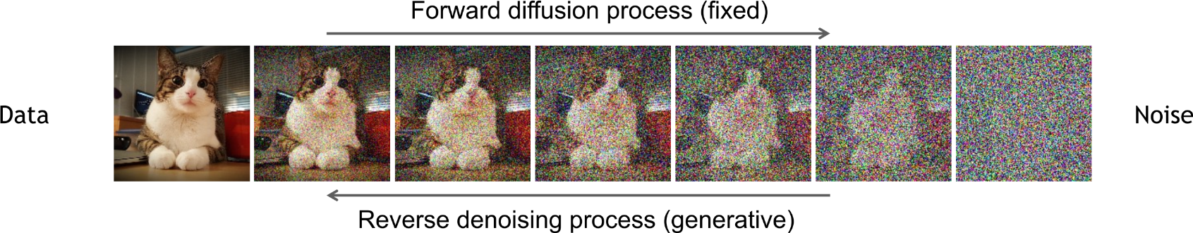
Forward Diffusion & Denoising
Visualizing Flow Matching Training
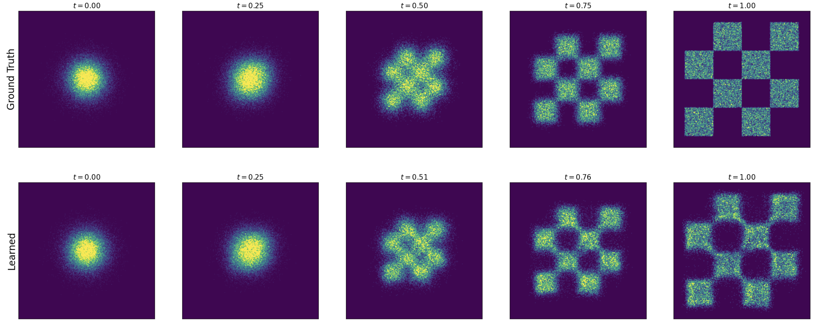
Training a flow matching model with Gaussian CondOT path. Top: ground truth marginal probability path \(p_t\). Bottom: samples from trained flow matching model. After training, the distributions match. From Holderrieth and Erives (2025).
Score Field Comparison
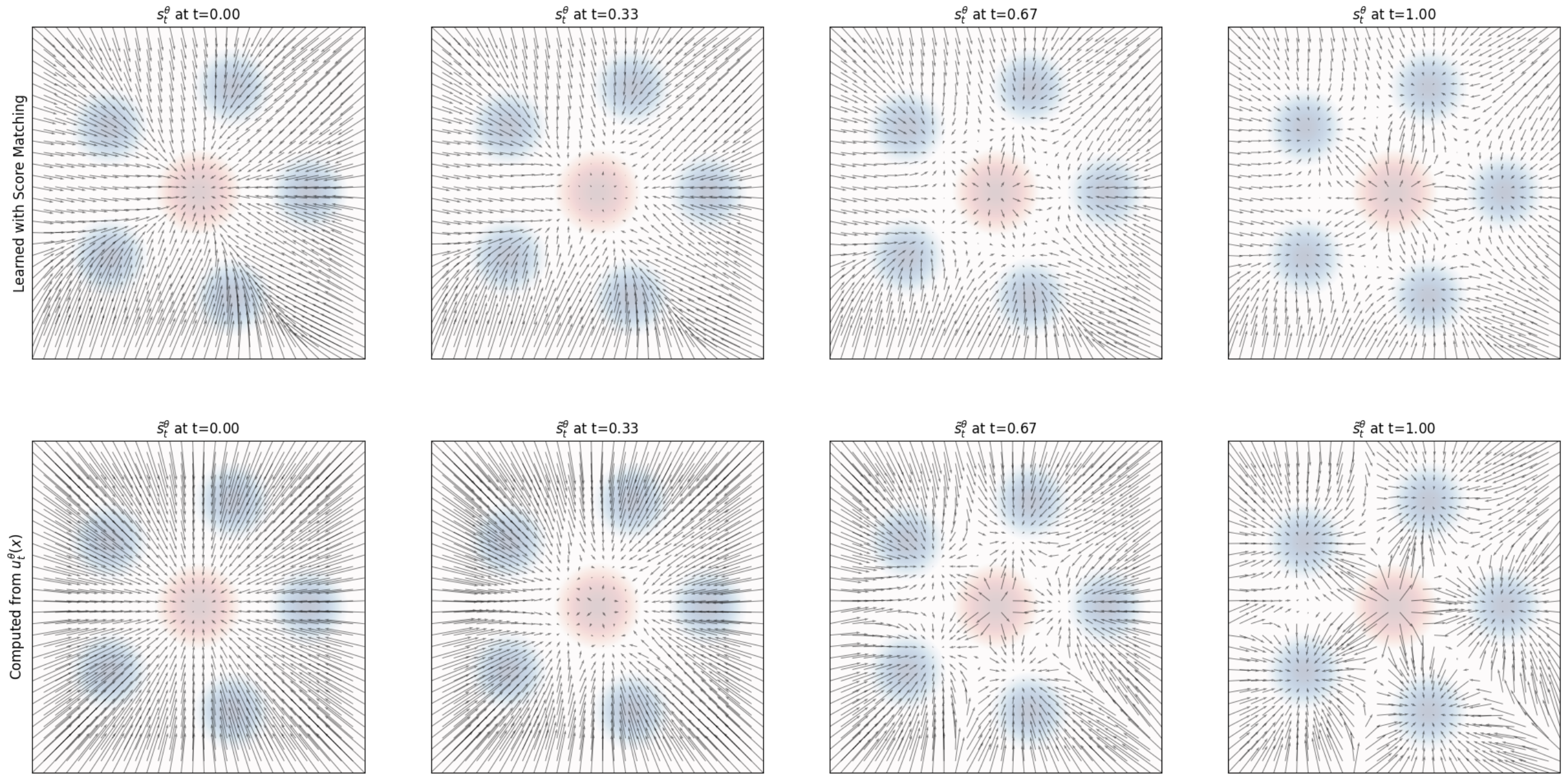
Top: Score field \(s_t^\theta(x)\) learned via score matching. Bottom: Score field derived from \(u_t^\theta\) via conversion formula. Both agree, confirming equivalence. From Holderrieth and Erives (2025).
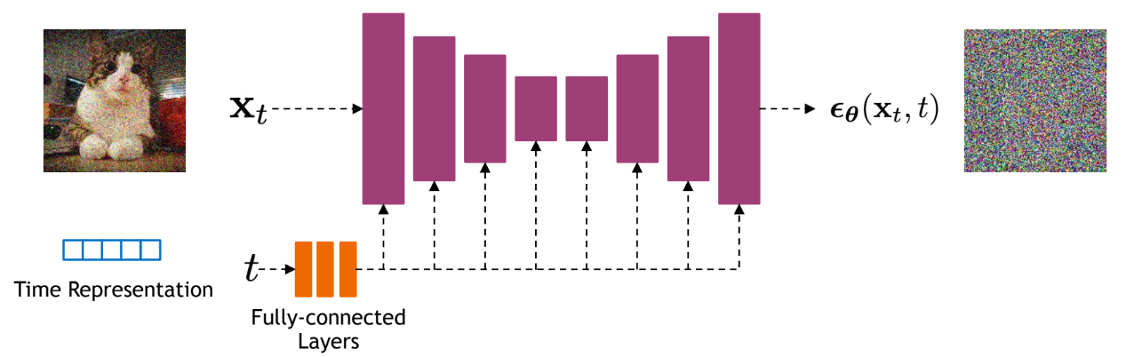
Neural Network Architecture
The neural network \(u_t^\theta(x \mid y)\) must accept:
- \(x \in \mathbb{R}^d\) (noised input)
- \(t \in [0,1]\) (time)
- \(y \in \mathcal{Y}\) (conditioning)
Common architectures:
- U-Net for images (convolutional)
- Diffusion Transformer (DiT) – attention-based