where \(\text{cov}(\boldsymbol{x}_f, \boldsymbol{y}_f) = \mathbb{E}\big[(\boldsymbol{x}_f - \boldsymbol{\mu}_f)(\boldsymbol{y}_f - \boldsymbol{\mu}_y)^T\big]\) is the cross-covariance and \(\text{cov}(\boldsymbol{y}_f) = \text{cov}(\boldsymbol{y}_f, \boldsymbol{y}_f)\).
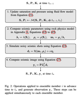
where \(\boldsymbol{S}^n\), \(\boldsymbol{P}^n\) = spatially discretized CO2 saturation and pressure at time \(t_n\), \(\boldsymbol{K}\) = permeability field, \(\boldsymbol{\phi}\) = porosity field, and \(\mathcal{M}\) = nonlinear operator that numerically solves the two-phase flow PDE from \(t_n\) to \(t_{n+1}\).
Solved numerically with JutulDarcy.jl (implicit Euler, Newton’s method, auto-diff).
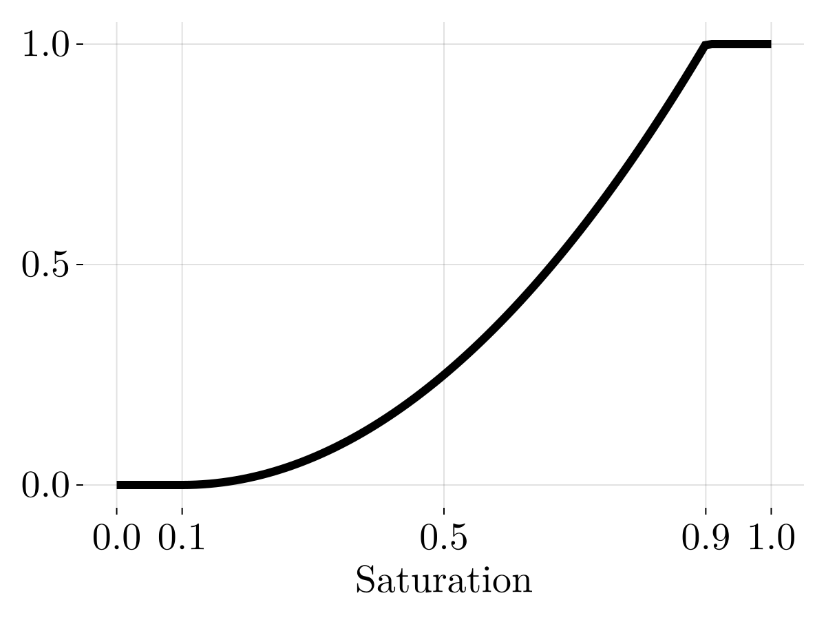
Relative Permeability Model
Modified Brooks-Corey model with residual saturation \(r\):
\(\mathbf{J}_0 = \frac{d\mathcal{H}}{d\boldsymbol{m}_0}(\boldsymbol{m}_0, \boldsymbol{\rho}_0)\): Jacobian of wave operator \(\mathcal{H}\) at smooth baseline model \((\boldsymbol{m}_0, \boldsymbol{\rho}_0)\)
\(\mathbf{P}\): linear post-processor that mutes the water layer and scales the image as a function of depth
\(\nu\): noise scaling parameter controlling SNR \(= -20\log\nu\) dB
\(\nu_B^*\): true noise magnitude for baseline survey
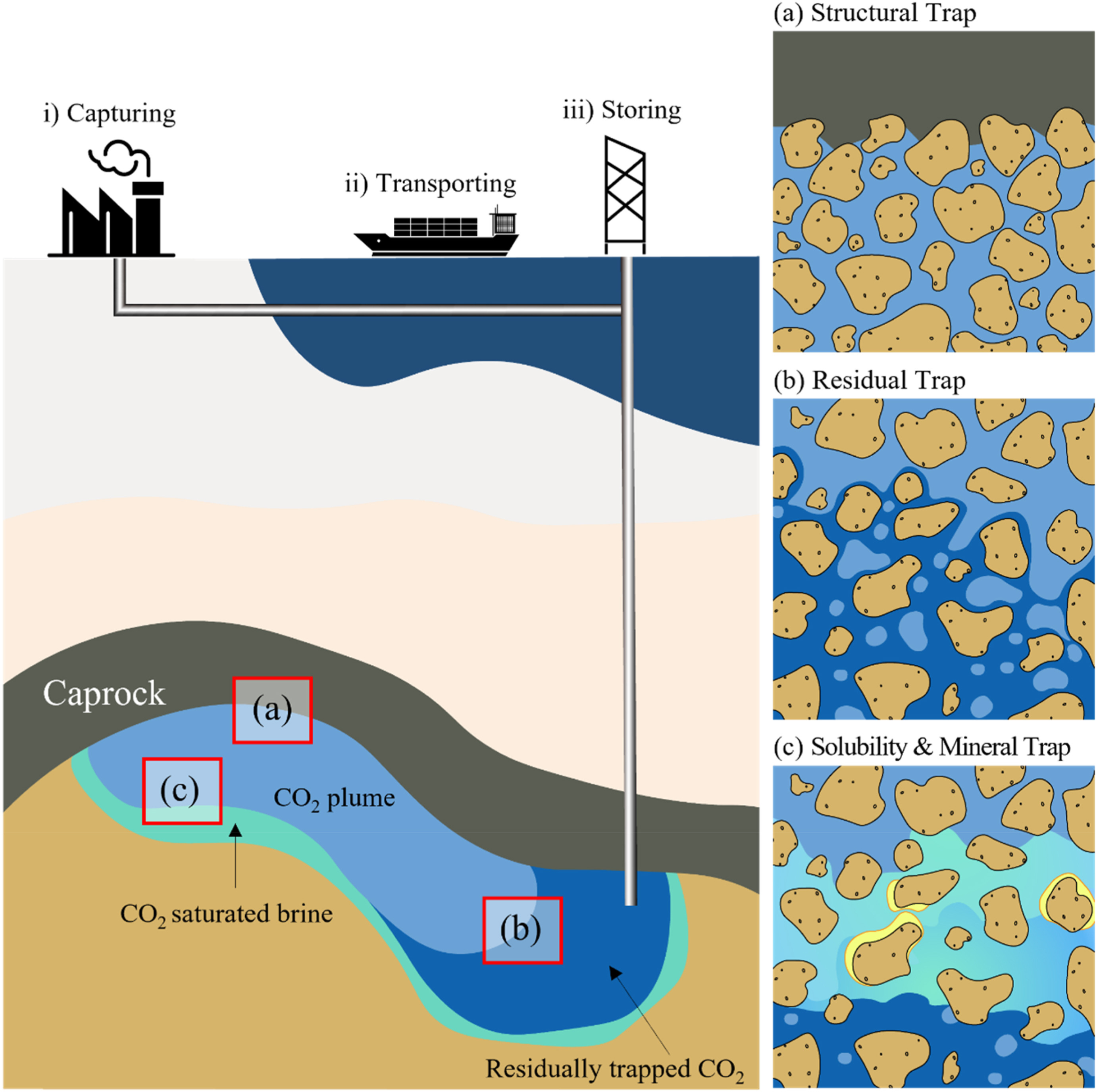
Baseline subtraction reveals changes due to CO2 injection.
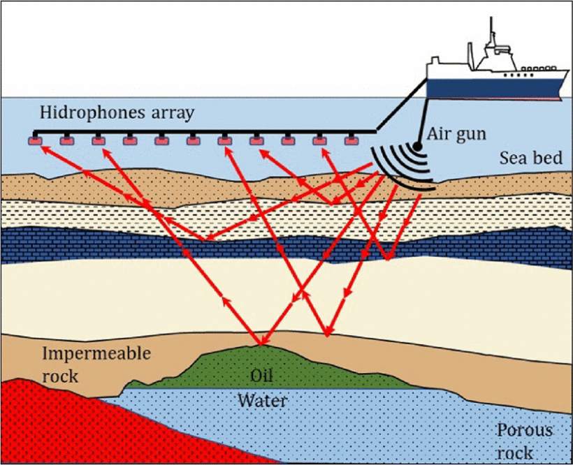
Seismic observation overview
Lots of data!
Each seismic source outputs a wave.
Each seismic receiver records a wave from each source.
Data size is product of
# of receivers,
# of sources,
# of waveform time steps.
Saraiva et al. (2021)
Time-lapse — pre-injection image
Baseline survey before injection: \(d_B\).
Approximate subsurface seismic parameters smoothly as \(m_0\): \(d_0 = F(m_0)\).
Gradient of misfit \(\|d_B - F(m_0)\|^2\)\(\implies\) seismic image \(A_B\).
Baseline survey
Time-lapse — post-injection image
Survey after injecting for some time: \(d\).
Difference in measurements: \(d - d_B\) (difficult to interpret).
Gradient of misfit \(\|d - F(m_0)\|^2\)\(\implies\) seismic image \(A\).
Monitor survey
Time-lapse — difference image
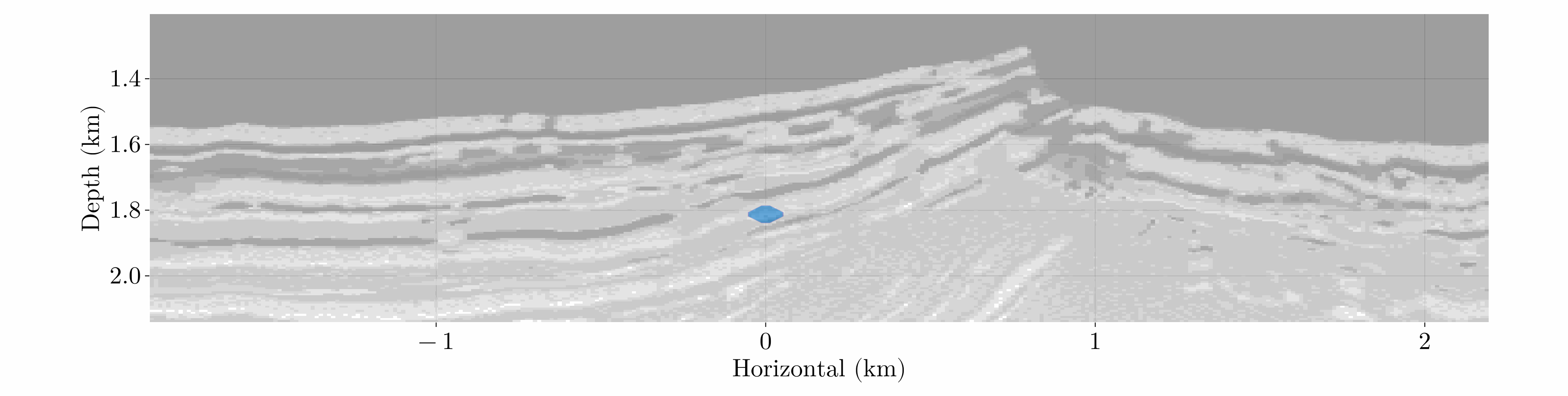
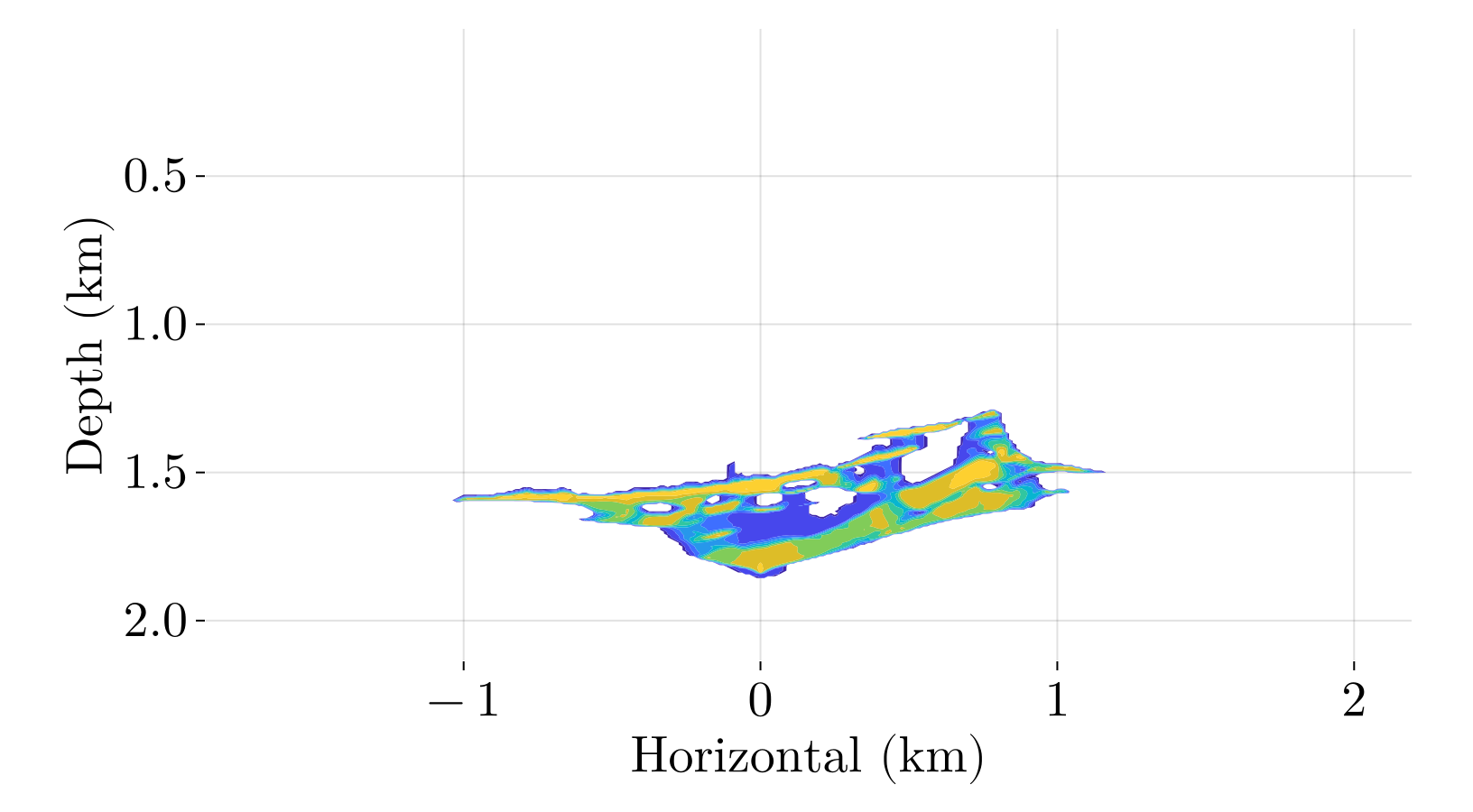
Example CO2 plume
Workflow Diagram
flowchart TB
    subgraph silico ["In Silico (simulation)"]
        A["Generate initial ensemble<br/>i = 1 to N_e with permeability estimates"] --> B
        B["S_i, P_i, K_i at time t_(n-1)<br/>conditioned on y^(1:n-1)"]
        B --> C["For each member, simulate<br/>flow to t_n and seismic survey"]
        C --> D["S_i, P_i, K_i, y_i at time t_n<br/>conditioned on y^(1:n-1)"]
        D --> E["Update ensemble based<br/>on survey at time t_n"]
        E --> F["S_i, P_i, K_i at time t_n<br/>conditioned on y^(1:n)"]
        F -->|"increment n"| B
    end
    subgraph situ ["In Situ (field)"]
        G["Set up injection site"] --> H
        H["Let time pass to t_n<br/>Conduct seismic survey"]
        H --> I["May use estimates for<br/>future injection decisions"]
        I -->|"increment n"| H
    end
    H -.->|"field survey y^n"| E
    F -.->|"estimates"| I

    style silico fill:#f0f4ff,stroke:#333
    style situ fill:#fff4f0,stroke:#333
\(\mathbf{R}\) acts as a regularization in the inversion and is a non-singular approximation of the covariance of any observation noise not already represented in \(\widehat{\text{cov}}(\mathbf{y}_f)\).
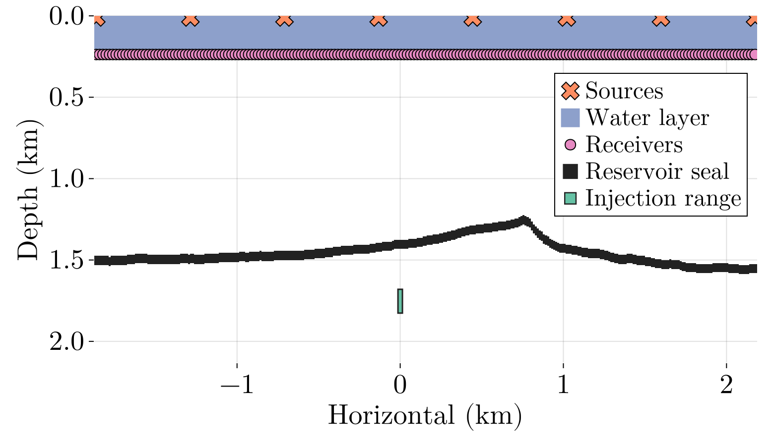
4.05 km \(\times\) 2.125 km on a 325 \(\times\) 341 grid
Cell size: 12.5 m \(\times\) 6.25 m
5-year injection, surveys every year
8 sources, 200 receivers
SNR = 8 dB
\(N_e = 256\) ensemble members
Based on 2D slice of Compass model (North Sea)
Seismic Field Parameters
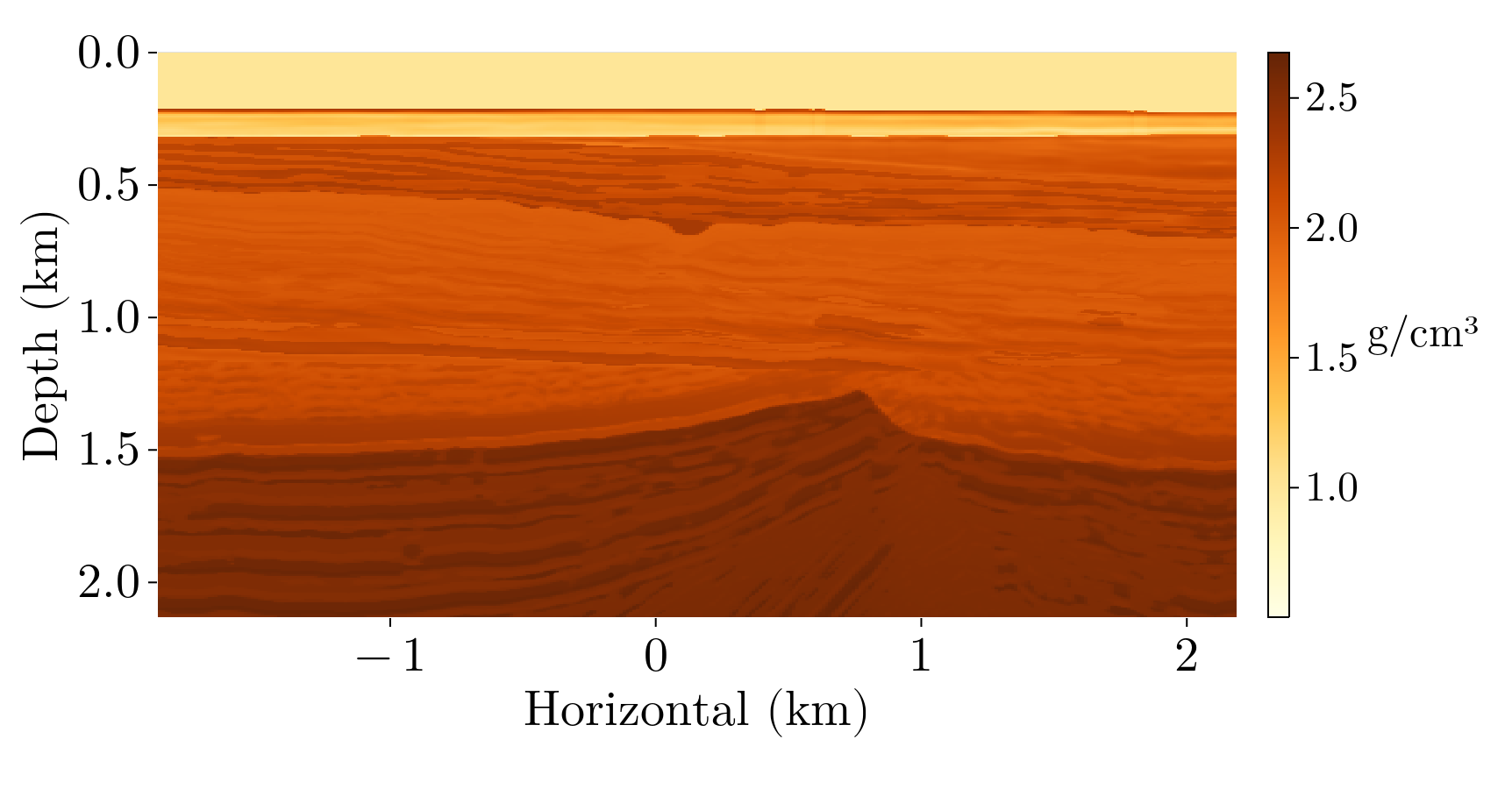
Density field
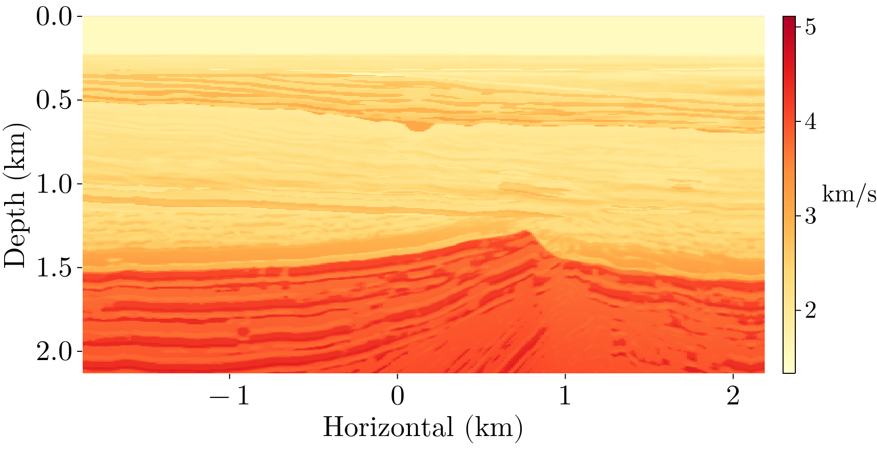
P-wave velocity field
Derived from a 2D slice of the Compass model, capturing geological complexity of the North Sea subsurface.
Permeability Ensemble
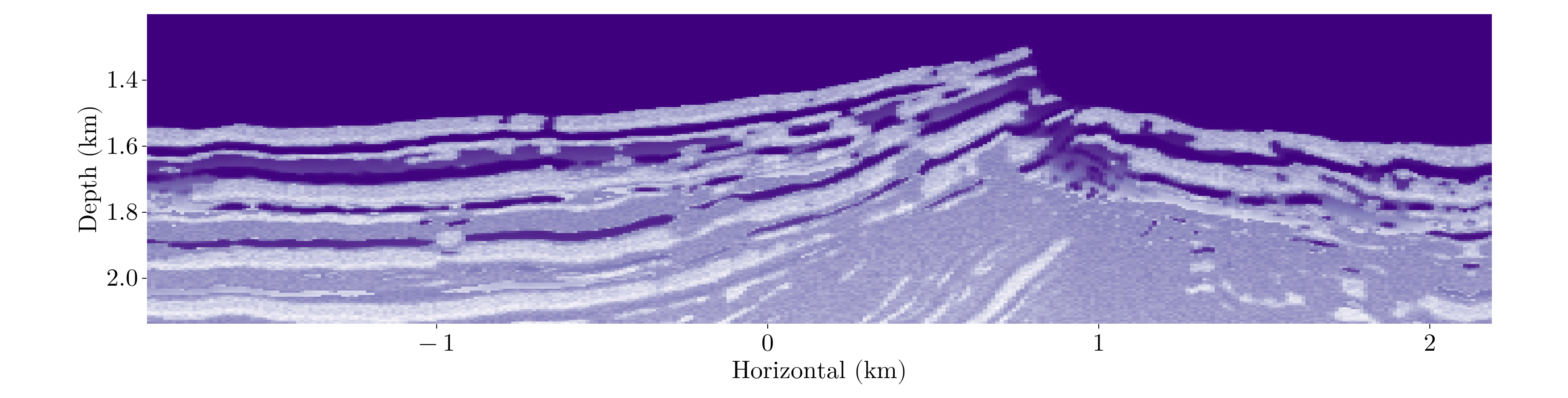
Ground-truth permeability field
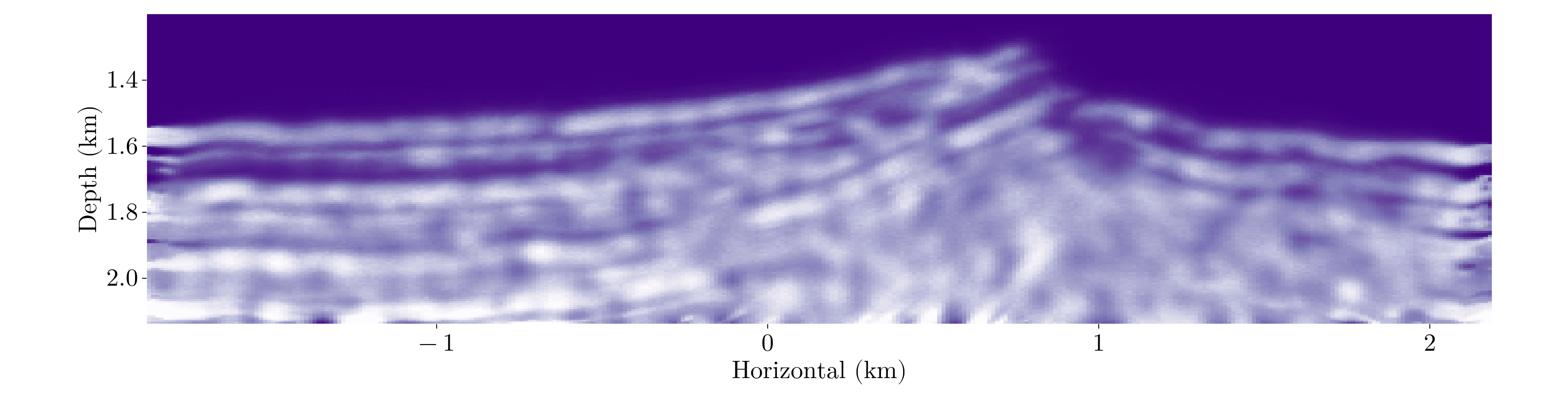
Ensemble mean
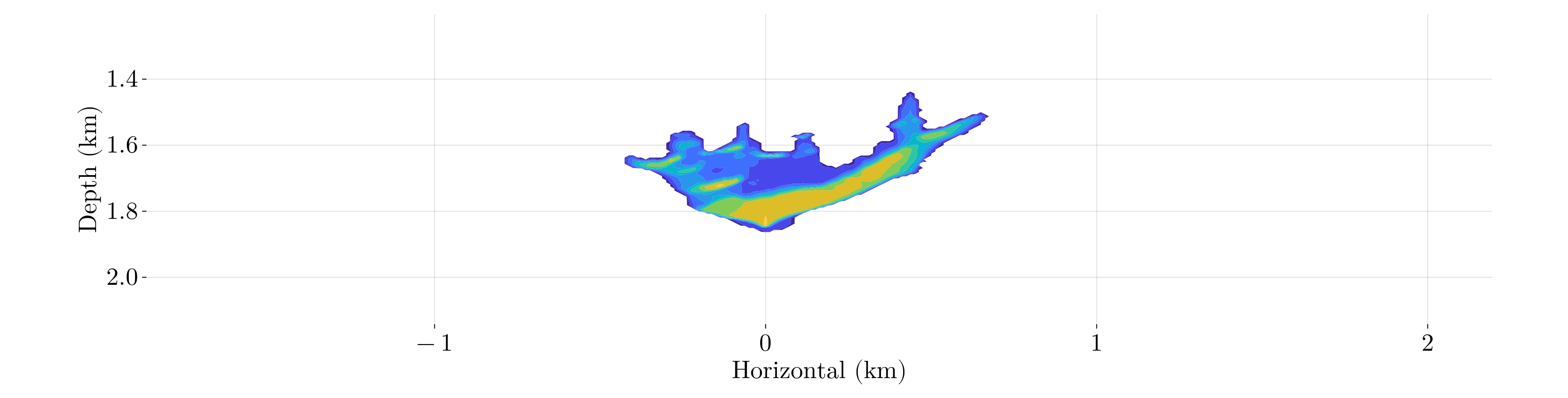
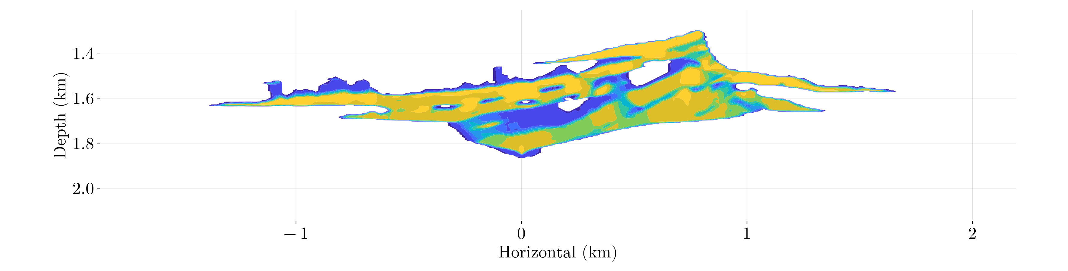
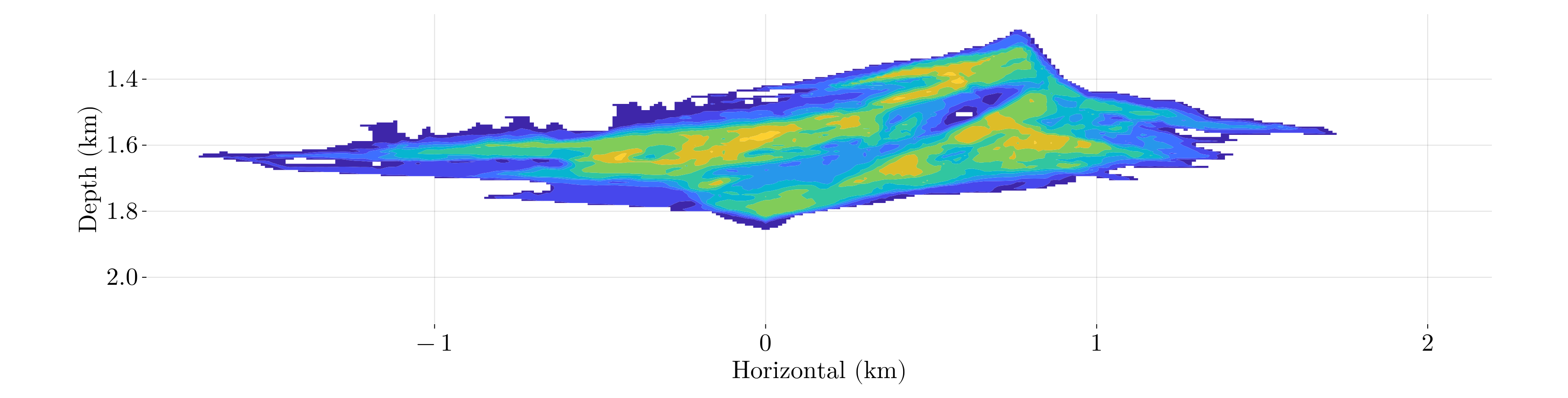
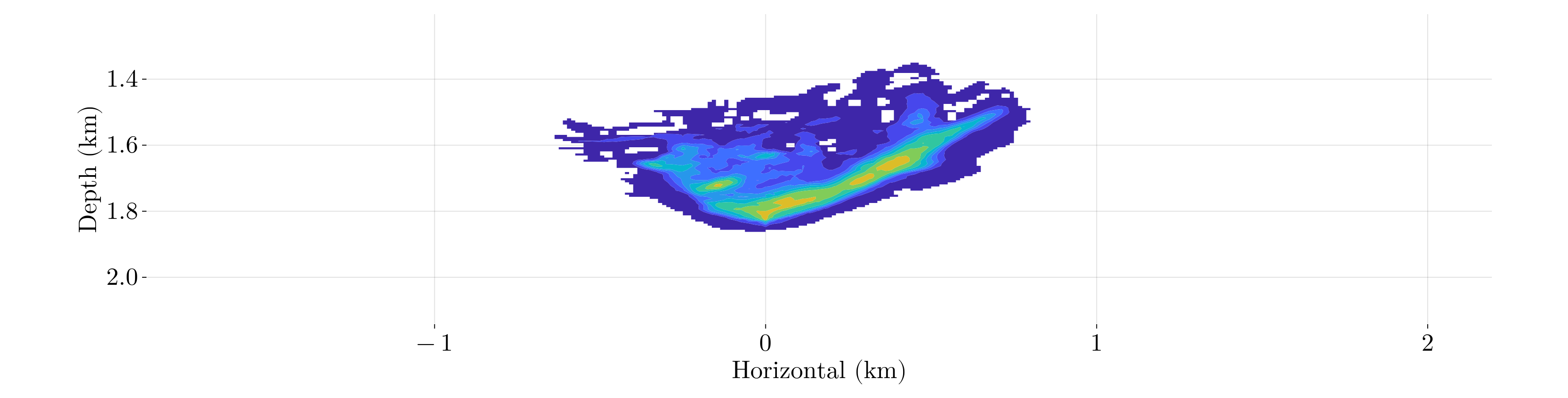
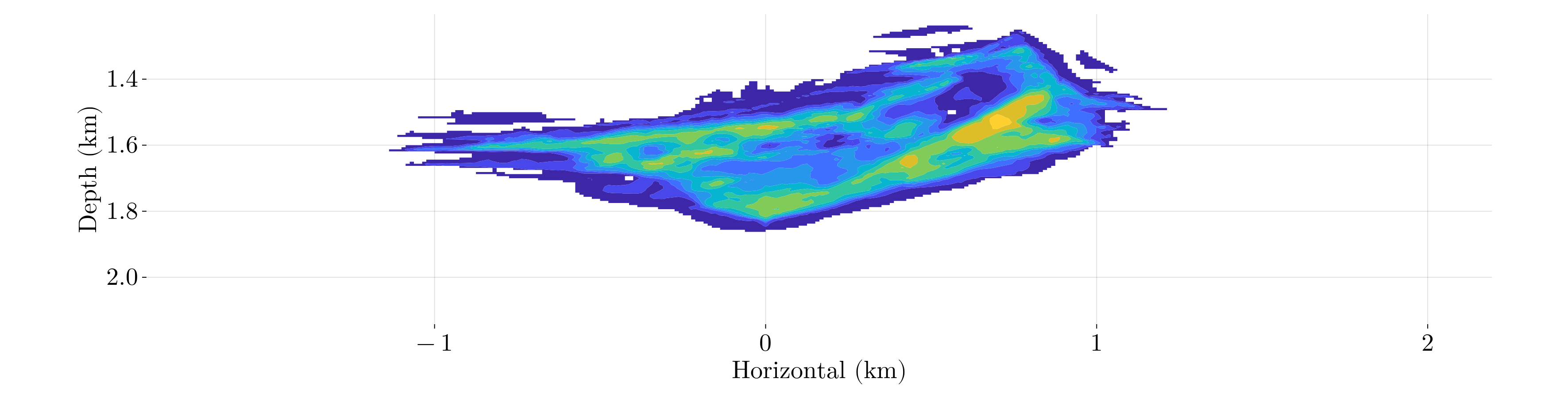
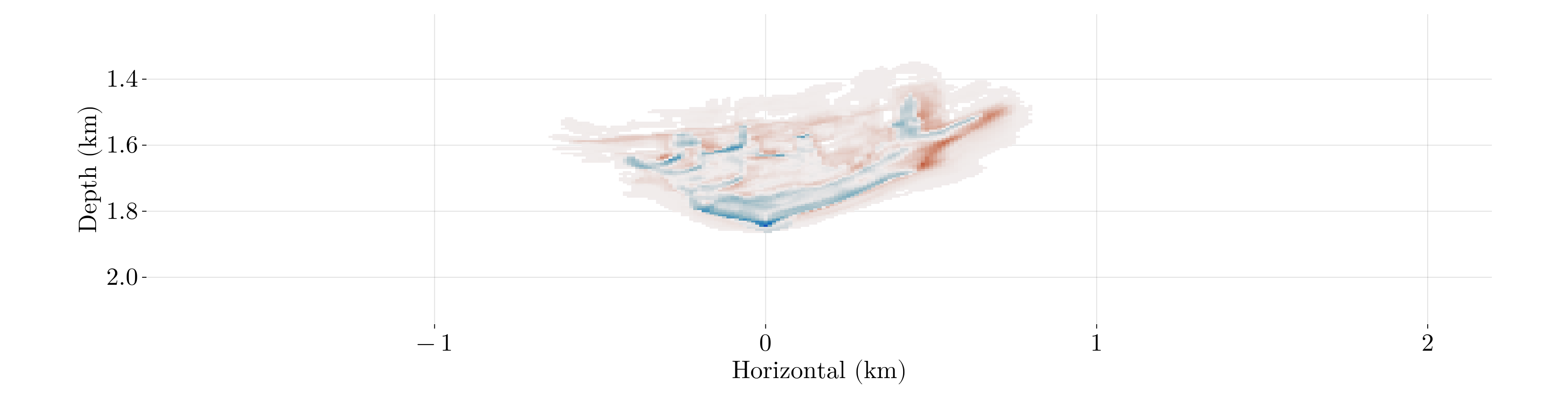
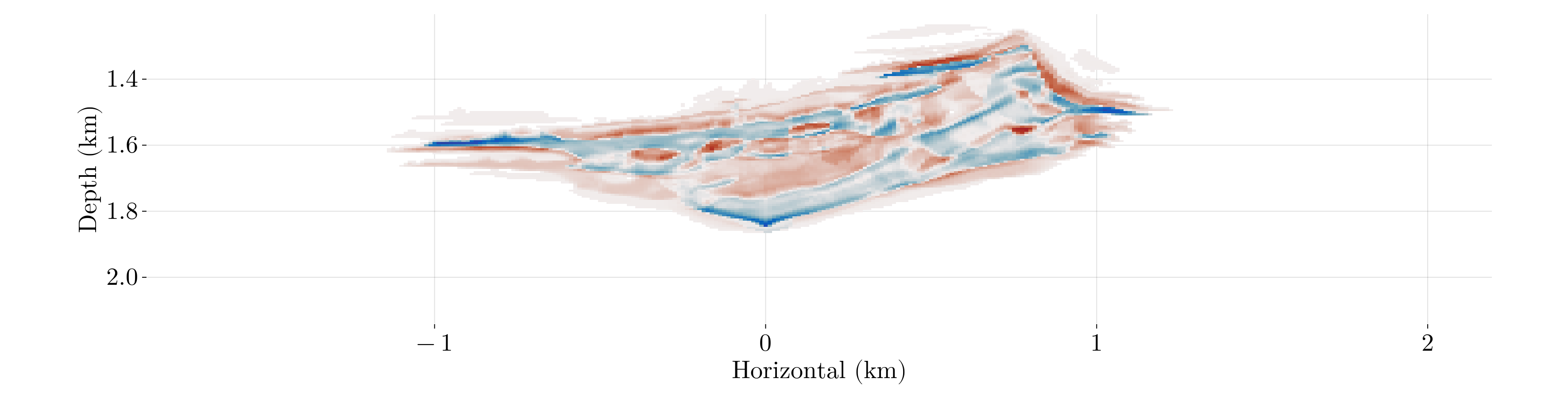
Ground-Truth CO2 Plume Evolution
CO2 saturation at year 1
CO2 saturation at year 5
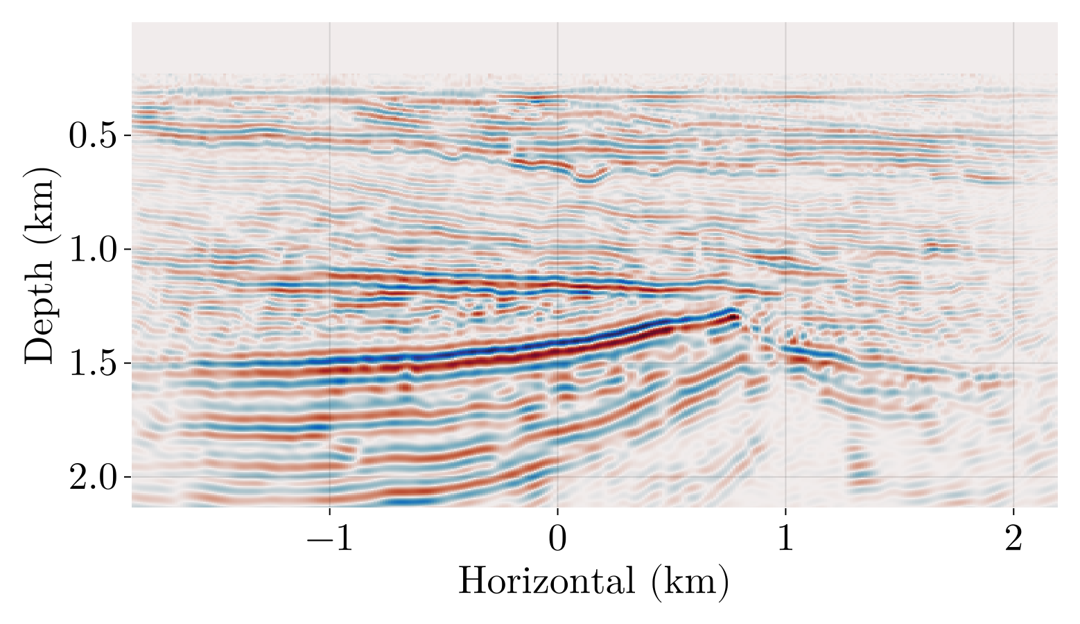
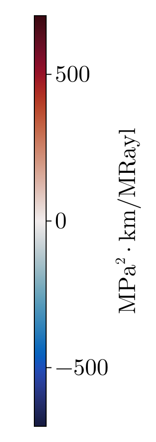
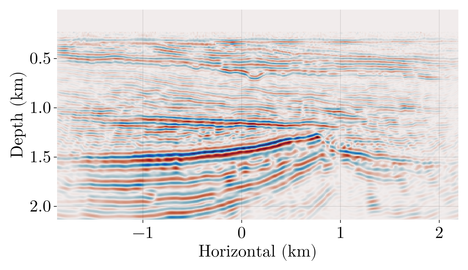
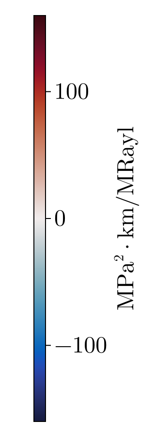
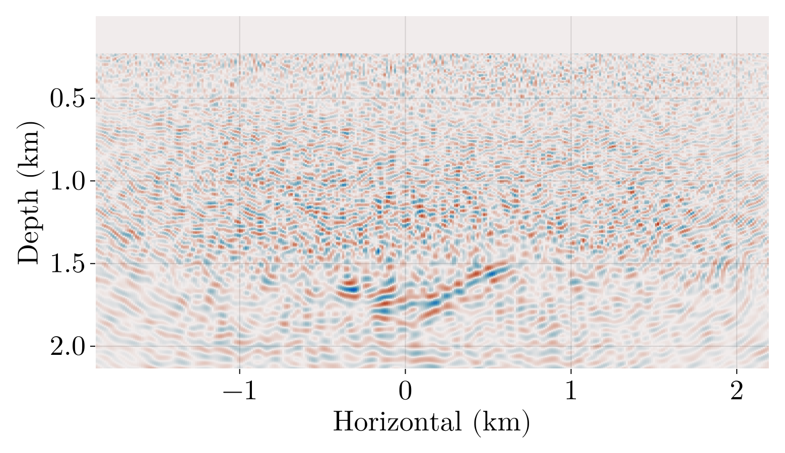
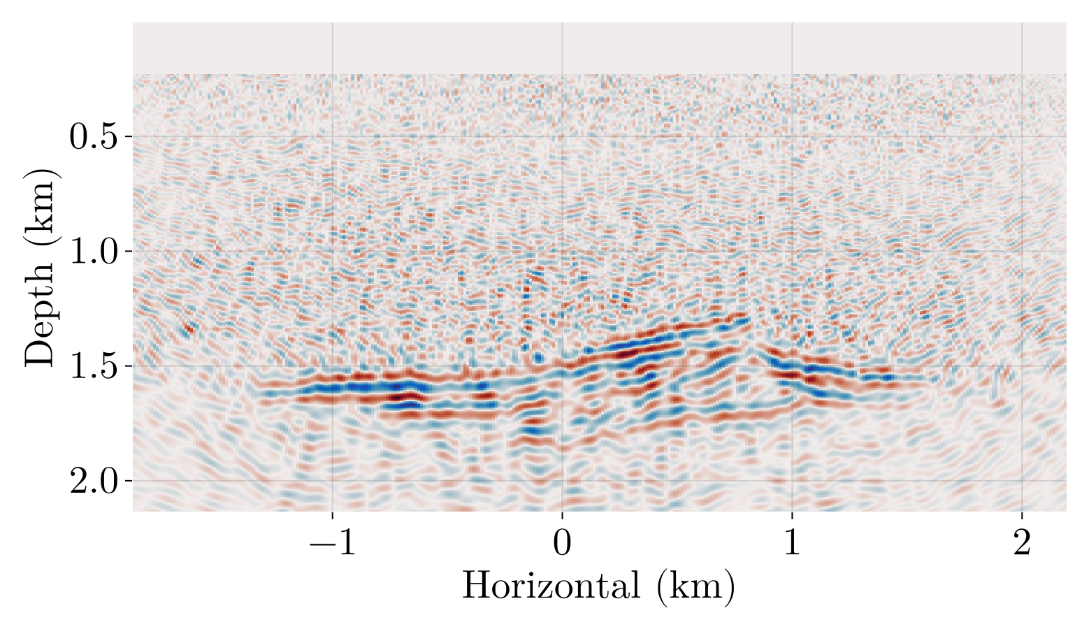
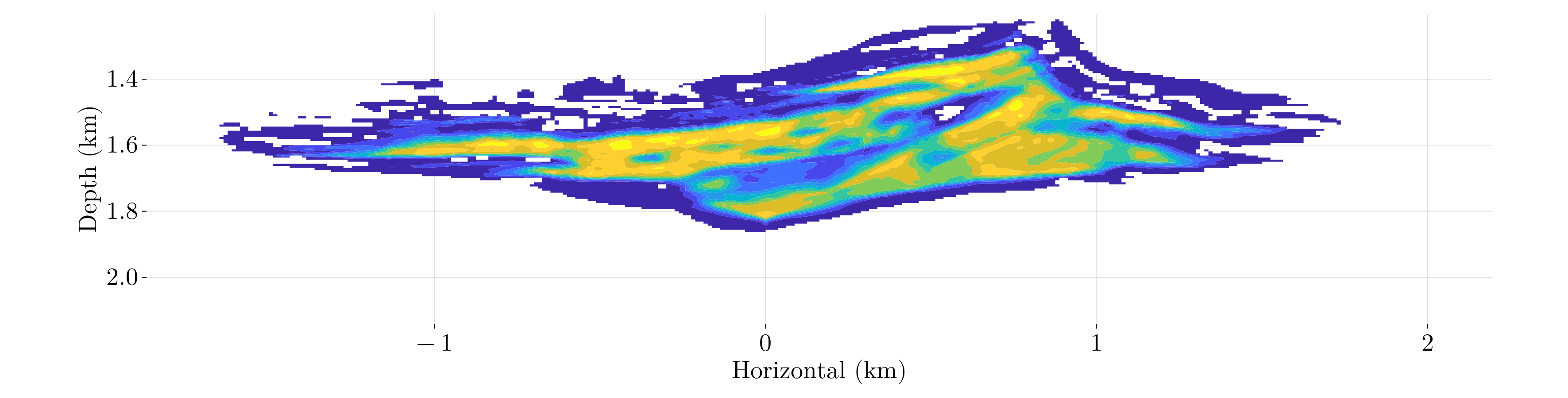
RTM image at year 1
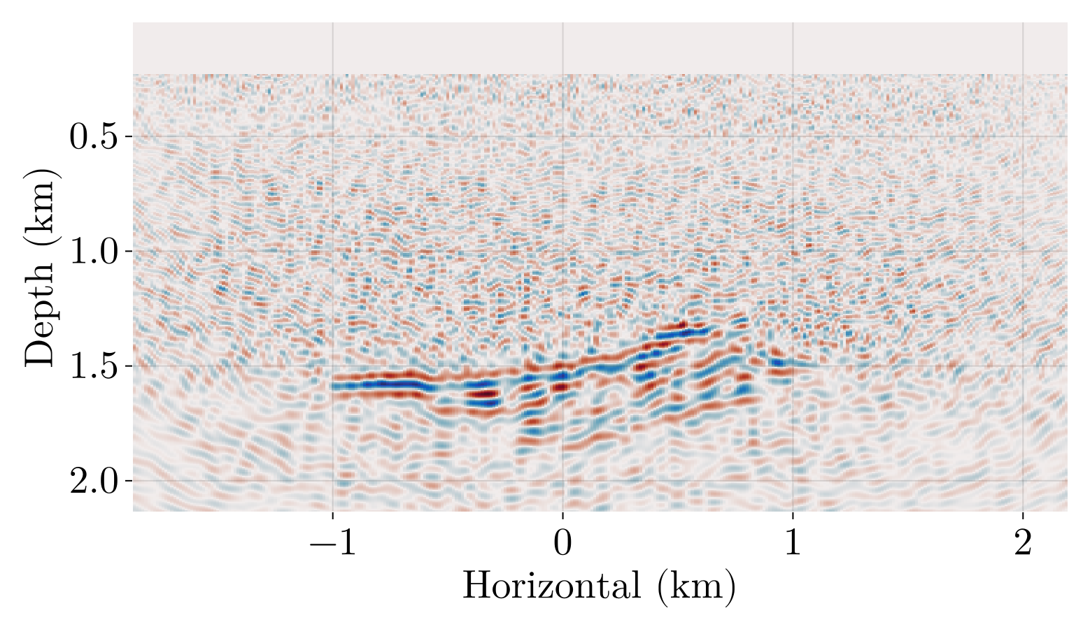
RTM image at year 5
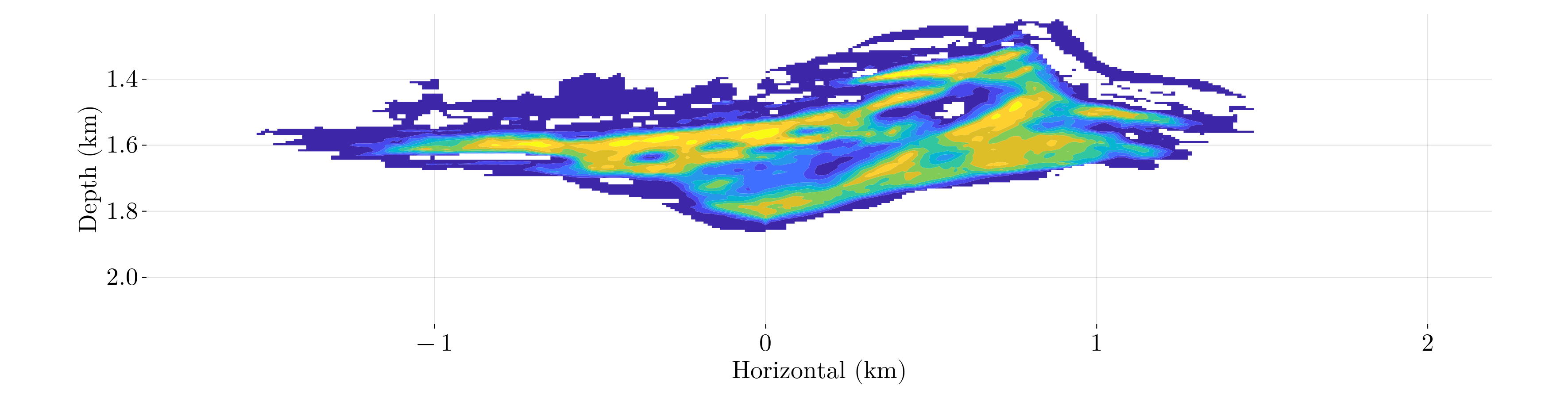
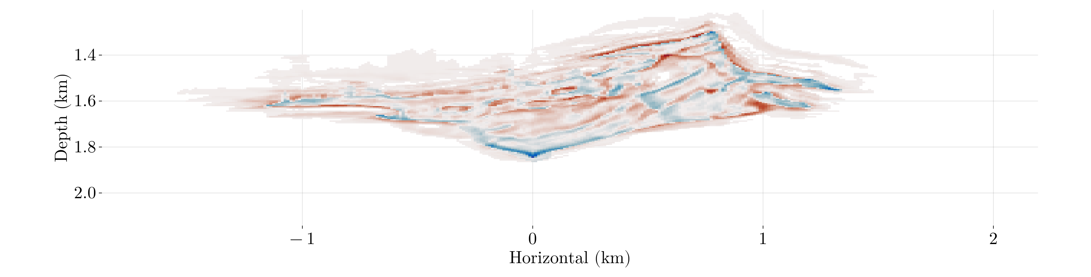
Results: EnKF vs. Baselines — Plume Estimates
Ground truth at year 5
NoObs prediction at year 5 (no surveys)
Ground truth at year 5
EnKF analysis at year 5 (five yearly surveys)
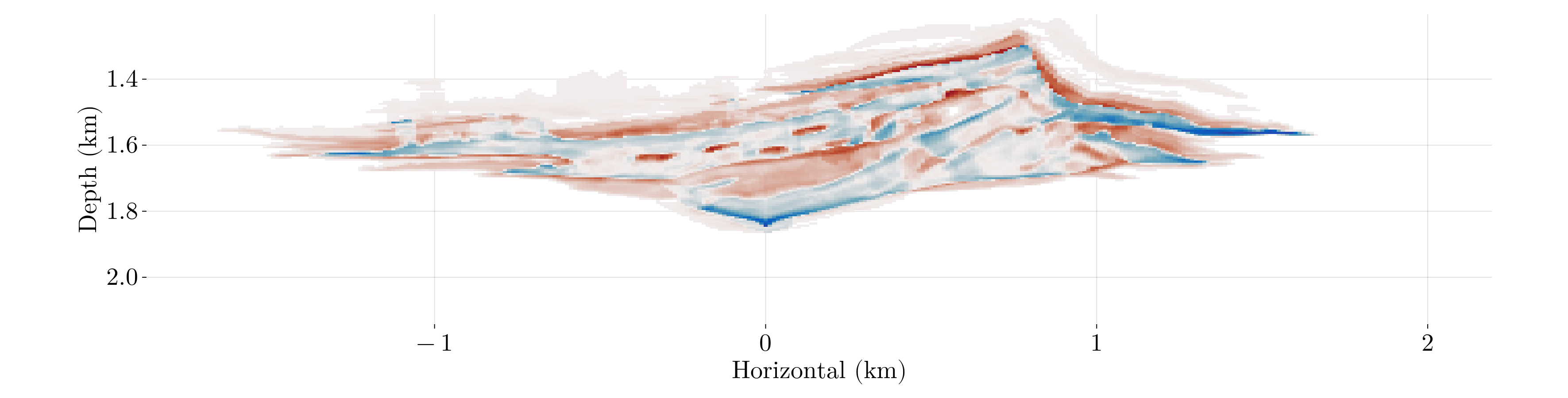
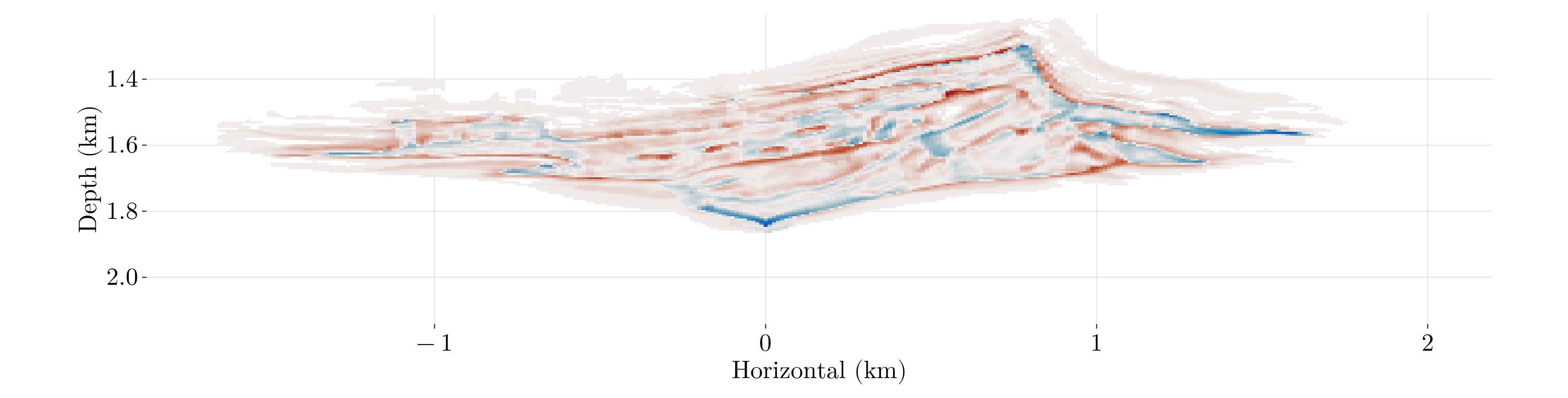
Results: Error Fields at Year 5
EnKF prediction error (4 surveys)
EnKF analysis error (5 surveys)
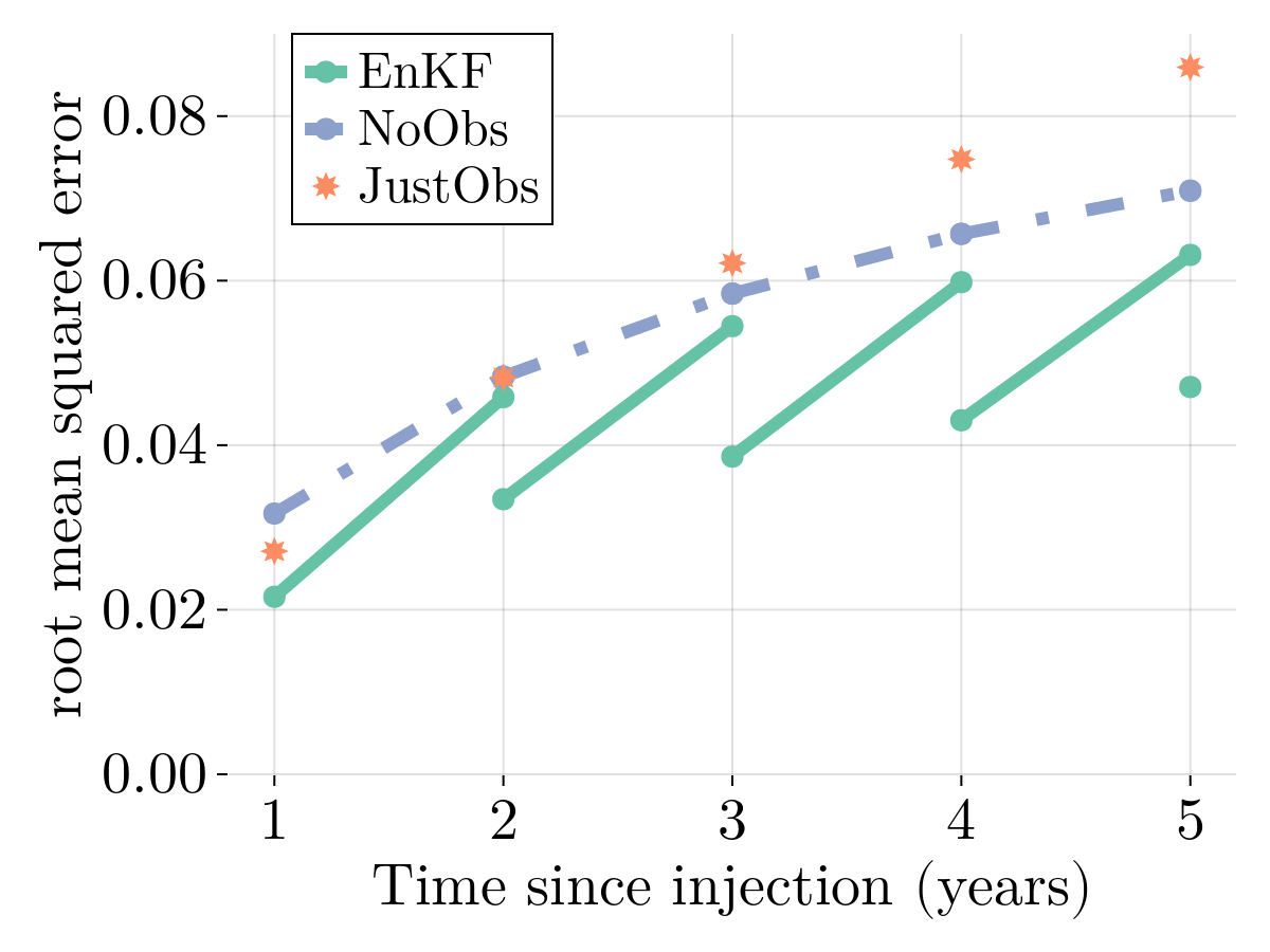
Results: Error Over Time
RMSE over time for all three methods
Key observations:
EnKF consistently achieves lower error than both baselines
NoObs error grows steadily due to permeability uncertainty
JustObs (even noise-free!) performs worse — dynamics are more informative than observations alone
Sharp drops at each yearly survey show the value of data assimilation
Error growth between surveys shows limits of forecasting with uncertain permeability
EnKF Plume Tracking Over Time
EnKF mean saturation
Year 3
Year 6
Year 9
Error
Year 3 error
Year 6 error
Year 9 error
Scalability Considerations
Current 2D experiment:
State vector: \(\sim 10^5\) DOF
Observation vector: \(\sim 10^6\) DOF
256 ensemble members
Scaling to 3D (\(\sim 10^{10}\,\text{m}^3\)):
State: \(\sim 10^7\) DOF
Standard KF: \(> 1\) TB storage
EnKF scales linearly with DOF
Ensemble size independent of grid size
Transition + observation trivially parallelizable
Cost perspective
The computational cost of the EnKF update is negligible compared to simulating transition and observation. And simulations are far cheaper than conducting a seismic survey.
Conclusions
EnKF + full waveform data + CO2 dynamics achieves lower error than either physics-only or observation-only baselines
The EnKF provides a scalable framework for seismic CO2 monitoring as a digital shadow
Update permeability (not just saturation) during assimilation
Currently the dominant source of forecast error
Use nonlinear seismic observations (move beyond Born approximation)
Include heterogeneous porosity and capillary pressure
Account for environmental noise (non-Gaussian, spatially correlated)
Explore ML-based DA with full waveform data (conditional normalizing flows)
Scale to 3D field-scale reservoirs
Ongoing work
See Gahlot et al. (2024) for preliminary results combining ML-based DA with full-waveform seismic data and CO2 fluid dynamics using conditional normalizing flows.
References
Bruer, Grant, Abhinav Prakash Gahlot, Edmond Chow, and Felix Herrmann. 2025. “Seismic Monitoring of CO2 Plume Dynamics Using Ensemble Kalman Filtering.”IEEE Transactions on Geoscience and Remote Sensing.
Thank You
Key takeaway: The ensemble Kalman filter is a promising, scalable approach for building digital shadows of subsurface CO2 reservoirs monitored with time-lapse seismic data.