Variational Data Assimilation

Data Assimilation

2024-01-29

Data Assimilation

Definition 1 Data assimilation (DA) is the approximation of the true state of some physical system at a given time, by combining time-distributed observations with a dynamic model in an optimal way.

DA is an approach for solving a specific class of inverse, or parameter estimation problems, where the parameter we seek is the initial condition.

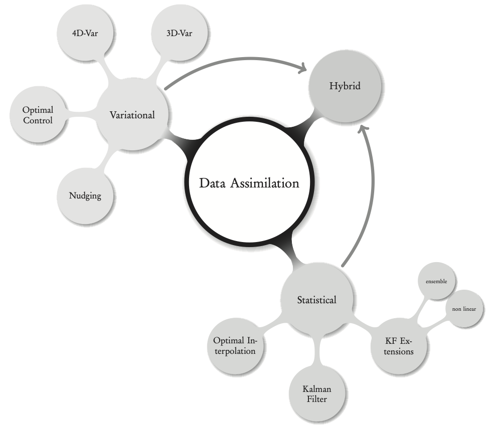
DA can be classically approached in two ways:

• variational DA
• statistical DA

Outline

Adjoint methods and variational data assimilation (4h)

1. Introduction to data assimilation: setting, history, overview, definitions.

2. Adjoint method.

3. Variational data assimilation methods:

   1. 3D-Var,

   2. 4D-Var.

Statistical estimation, Kalman filters and sequential data assimilation (4h)

Introduction to statistical DA.

Statistical estimation.

The Kalman filter.

Nonlinear extensions and ensemble filters.

Reference Text Books

Overview

From Asch (2022)

Variational DA—formulation

In variational data assimilation we describe the state of the system by

• a state variable, \(\mathbf{x}(t)\in\mathcal{X},\) a function of space and time that

• represents the physical variables of interest, such as current velocity (in oceanography), temperature, sea-surface height, salinity, biological species concentration, chemical concentration, etc.

Evolution of the state is described by a system of (in general nonlinear) differential equations in a region \(\Omega,\) \[\left\{ \begin{aligned} & \frac{\mathrm{d}\mathbf{x}}{\mathrm{d}t}=\mathcal{M}(\mathbf{x})\quad\mathrm{in}\;\Omega\times\left[0,T\right],\\ & \mathbf{x}(t=0)=\mathbf{x}_{0}, \end{aligned} \right. \tag{1}\] where the initial condition is unknown (or poorly known).

Suppose that we are in possession of observations \(\mathbf{y}(t)\in\mathcal{O}\) and an observation operator \(\mathcal{H}\) that describes the available observations.

Then, to characterize the difference between the observations and the state, we define the objective (or cost) function, \[J(\mathbf{x}_{0})=\frac{1}{2}\int_{0}^{T}\left\Vert \mathbf{y}(t)-\mathcal{H}\left(\mathbf{x}(\mathbf{x}_{0},t)\right)\right\Vert _{\mathcal{O}}^{2}\mathrm{d}t+\frac{1}{2}\left\Vert \mathbf{x}_{0}-\mathbf{x}^{\mathrm{b}}\right\Vert _{\mathcal{X}}^{2} \tag{2}\] where

• \(\mathbf{x}^{\mathrm{b}}\) is the background (or first guess)

• and the second term plays the role of a regularization (in the sense of Tikhonov see previous Lecture.

• The two norms under the integral, in the finite-dimensional case, will be represented by the error covariance matrices \(\mathbf{R}\) and \(\mathbf{B}\) respectively, and will be described below.

• Note that for mathematical rigor we have indicated, as subscripts, the relevant functional spaces on which the norms are defined.

In the continuous context, the data assimilation problem is formulated as follows:

Important

Find the analyzed state \(\mathbf{x}^a_0\) that minimizes \(J\) and satisfies

\[\mathbf{x}^a_0=\mathop{\mathrm{arg\,min}}_{\mathbf{x}_0} J(\mathbf{x}_0)\]

The necessary condition for the existence of a (local) minimum is (as usual...) \[\nabla J(\mathbf{x}_{0}^{\mathrm{a}})=0.\]

Variational DA is based on an adjoint approach that is explained in the previous Lecture.

The particularity here is that the adjoint is used to solve an inverse problem for the unknown initial condition.

Variational DA—3D Var

Usually, 3D-Var and 4D-Var are introduced in a finite dimensional or discrete context this approach will be used in this section.

For the infinite dimensional or continuous case, we must use the calculus of variations and (partial) differential equations, as was done in the previous Lectures.

We start out with the finite-dimensional version of the cost function 2, \[\begin{aligned} J(\mathbf{x}) & =\frac{1}{2}\left(\mathbf{x}-\mathbf{x}^{\mathrm{b}}\right)^{\mathrm{T}}\mathbf{B}^{-1}\left(\mathbf{x}-\mathbf{x}^{\mathrm{b}}\right)\\ & +\frac{1}{2}\left(\mathbf{Hx}-\mathbf{y}\right)^{\mathrm{T}}\mathbf{R}^{-1}\left(\mathbf{Hx}-\mathbf{y}\right), \end{aligned} \tag{3}\] where

• \(\mathbf{x},\) \(\mathbf{x}^{\mathrm{b}},\) and \(\mathbf{y}\) are the state, the background state, and the measured state respectively;

• \(\mathbf{H}\) is the observation matrix (a linearization of the observation operator \(\mathcal{H}\) );

• \(\mathbf{R}\) and \(\mathbf{B}\) are the observation and background error covariance matrices respectively.

This quadratic function attempts to strike a balance between some a priori knowledge about a background (or historical) state and the actual measured, or observed, state.

It also assumes that we know and that we can invert the matrices \(\mathbf{R}\) and \(\mathbf{B}\). This, as we will be pointed out below, is not always obvious.

Furthermore, it represents the sum of the (weighted) background deviations and the (weighted) observation deviations. The basic methodology is presented in the Algorithm below, which is nothing more than a classical gradient descent algorithm.

\(j=0\), \(x=x_{0}\)

while \(\left\Vert \nabla J\right\Vert >\epsilon\) or \(j\le j_{\mathrm{max}}\)

    compute \(J\)

    compute \(\nabla J\)

    gradient descent and update of \(x_{j+1}\)

    \(j=j+1\)

end

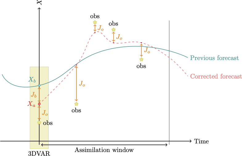
We note that when

• the background \(\mathbf{x}^{\mathrm{b}}=\mathbf{x}^{\mathrm{b}}+\epsilon^{\mathrm{b}}\) is available at some time \(t_{k},\) together with

• observations of the form \(\mathbf{y}=\mathbf{Hx}^{\mathrm{t}}+\epsilon^{\mathrm{o}}\) that have been acquired at the same time (or over a short enough interval of time when the dynamics can be considered stationary),

• then the minimization of 3 will produce an estimate of the system state at time \(t_{k}.\)

In this case, the analysis is called “three-dimensional variational analysis” and is abbreviated by 3D-Var.

Borrowing from control theory see Asch (2022) the optimal gain can be shown to take the form \[\mathbf{K}=\mathbf{B}\mathbf{H}^{\mathrm{T}}(\mathbf{H}\mathbf{B}\mathbf{H}^{\mathrm{T}}+\mathbf{R})^{-1},\] where \(\mathbf{B}\) and \(\mathbf{R}\) are the covariance matrices.

We obtain the analyzed state, \[\mathbf{x}^{\mathrm{a}}=\mathbf{x}^{\mathrm{b}}+\mathbf{K}(\mathbf{y}-\mathbf{H}(\mathbf{x}^{\mathrm{b}})).\]

This is the state that minimizes the 3D-Var cost function.

We can verify this by taking the gradient, term by term, of the cost function Equation 3 and equating to zero, \[\nabla J(\mathbf{x}^{\mathrm{a}})=\mathbf{B}^{-1}\left(\mathbf{x}^{\mathrm{a}}-\mathbf{x}^{\mathrm{b}}\right)-\mathbf{H}^{\mathrm{T}}\mathbf{R}^{-1}\left(\mathbf{y}-\mathbf{H}\mathbf{x}^{\mathrm{a}}\right)=0,\label{eq:gradJ3DVar}\]

where \[\mathbf{x}^{\mathrm{a}}=\mathop{\mathrm{arg\,min}}J(\mathbf{x}).\]

Solving the equation, we find \[\begin{aligned} \mathbf{B}^{-1}\left(\mathbf{x}^{\mathrm{a}}-\mathbf{x}^{\mathrm{b}}\right) & = & \mathbf{H}^{\mathrm{T}}\mathbf{R}^{-1}\left(\mathbf{y}-\mathbf{H}\mathbf{x}^{\mathrm{a}}\right)\nonumber \\ \left(\mathbf{B}^{-1}+\mathbf{H}^{\mathrm{T}}\mathbf{R}^{-1}\mathbf{H}\right)\mathbf{x}^{\mathrm{a}}& = & \mathbf{H}^{\mathrm{T}}\mathbf{R}^{-1}\mathbf{y}+\mathbf{B}^{-1}\mathbf{x}^{\mathrm{b}}\nonumber \\ \mathbf{x}^{\mathrm{a}}& = & \left(\mathbf{B}^{-1}+\mathbf{H}^{\mathrm{T}}\mathbf{R}^{-1}\mathbf{H}\right)^{-1}\left(\mathbf{H}^{\mathrm{T}}\mathbf{R}^{-1}\mathbf{y}+\mathbf{B}^{-1}\mathbf{x}^{\mathrm{b}}\right)\nonumber \\ & = & \left(\mathbf{B}^{-1}+\mathbf{H}^{\mathrm{T}}\mathbf{R}^{-1}\mathbf{H}\right)^{-1}\left(\left(\mathbf{B}^{-1}+\mathbf{H}^{\mathrm{T}}\mathbf{R}^{-1}\mathbf{H}\right)\mathbf{x}^{\mathrm{b}}\right.\nonumber \\ & ~ & \left.-\mathbf{H}^{\mathrm{T}}\mathbf{R}^{-1}\mathbf{H}\mathbf{x}^{\mathrm{b}}+\mathbf{H}^{\mathrm{T}}\mathbf{R}^{-1}\mathbf{y}\right)\nonumber \\ & = & \mathbf{x}^{\mathrm{b}}+\left(\mathbf{B}^{-1}+\mathbf{H}^{\mathrm{T}}\mathbf{R}^{-1}\mathbf{H}\right)^{-1}\mathbf{H}^{\mathrm{T}}\mathbf{R}^{-1}\left(\mathbf{y}-\mathbf{H}\mathbf{x}^{\mathrm{b}}\right)\nonumber \\ & = & \mathbf{x}^{\mathrm{b}}+\mathbf{K}\left(\mathbf{y}-\mathbf{H}\mathbf{x}^{\mathrm{b}}\right),\label{eq:lincontrol} \end{aligned} \tag{4}\]

where we have simply added and subtracted the term \(\left(\mathbf{H}^{\mathrm{T}}\mathbf{R}^{-1}\mathbf{H}\right)\mathbf{x}^{\mathrm{b}}\) in the third-last line and in the last line we have brought out what are known as the innovation term, \[\mathbf{d}=\mathbf{y}-\mathbf{H}\mathbf{x}^{\mathrm{b}},\] and the gain matrix, \[\mathbf{K}=\left(\mathbf{B}^{-1}+\mathbf{H}^{\mathrm{T}}\mathbf{R}^{-1}\mathbf{H}\right)^{-1}\mathbf{H}^{\mathrm{T}}\mathbf{R}^{-1}.\]

This matrix can be rewritten as \[\mathbf{K}=\mathbf{B}\mathbf{H}^{\mathrm{T}}\left(\mathbf{R}+\mathbf{H}\mathbf{B}\mathbf{H}^{\mathrm{T}}\right)^{-1} \tag{5}\]

using a well-known Sherman-Morrison-Woodbury formula of linear algebra that completely avoids the direct computation of the inverse of the matrix \(\mathbf{B}.\)

The linear combination in 4 of a background term plus a multiple of the innovation is a classical result of linear-quadratic (LQ) control theory and shows how nicely DA fits in with and corresponds to (optimal) control theory

The form of the gain matrix 5 can be explained quite simply.

• The term \(\mathbf{H}\mathbf{B}\mathbf{H}^{\mathrm{T}}\) is the background covariance transformed to the observation space.

• The “denominator” term \(\mathbf{R}+\mathbf{H}\mathbf{B}\mathbf{H}^{\mathrm{T}}\) expresses the sum of observation and background covariances.

• The “numerator” term \(\mathbf{B}\mathbf{H}^{\mathrm{T}}\) takes the ratio of \(\mathbf{B}\) and \(\mathbf{R}+\mathbf{H}\mathbf{B}\mathbf{H}^{\mathrm{T}}\) back to the model space.

This recalls (and is completely analogous to) the variance ratio

\[\frac{\sigma_{\mathrm{b}}^{2}}{\sigma_{b}^{2}+\sigma_{\mathrm{o}}^{2}}\] that appears in the optimal BLUE (Best Linear Unbiased Estimate) that will be derived later in the statistical DA Lecture.

This corresponds to the case of a single observation \(y^{\mathrm{o}}=x^{\mathrm{o}}\) of a quantity \(x,\) \[\begin{aligned} x^{\mathrm{a}} & = & x^{\mathrm{b}}+\frac{\sigma_{\mathrm{b}}^{2}}{\sigma_{\mathrm{b}}^{2}+\sigma_{\mathrm{o}}^{2}}(x^{\mathrm{o}}-x^{\mathrm{b}})\\ & = & x^{\mathrm{b}}+\frac{1}{1+\alpha}(x^{\mathrm{o}}-x^{\mathrm{b}}), \end{aligned}\]

where \[\alpha=\frac{\sigma_{\mathrm{o}}^{2}}{\sigma_{\mathrm{b}}^{2}}.\]

In other words, the best way to estimate the state is to take a weighted average of the background (or prior) and the observations of the state. And the best weight is the ratio of the mean squared errors (variances).

The statistical viewpoint is thus perfectly reproduced in the 3D-Var framework.

Variational DA — 4D Var

A more realistic, but complicated situation arises when one wants to assimilate observations that are acquired over a time interval, during which the system dynamics (flow, for example) cannot be neglected.

Suppose that the measurements are available at a succession of instants, \(t_{k},\) \(k=0,1,\ldots,K\) and are of the form \[\mathbf{y}_{k}=\mathbf{H}_{k}\mathbf{x}_{k}+\boldsymbol{\epsilon}^{\mathrm{o}}_{k}, \tag{6}\] where

• \(\mathbf{H}_{k}\) is a linear observation operator and

• \(\boldsymbol{\epsilon}^{\mathrm{o}}_{k}\) is the observation error with covariance matrix \(\mathbf{R}_{k},\)

• and suppose that these observation errors are uncorrelated in time.

Now we add the dynamics described by the state equation, \[\mathbf{x}_{k+1}=\mathbf{M}_{k+1}\mathbf{x}_{k}, \tag{7}\] where we have neglected any model error.¹

We suppose also that at time index \(k=0\) we know

• the background state \(\mathbf{x}^{\mathrm{b}}_{0}\) and

• its error covariance matrix \(\mathbf{P}^{\mathrm{b}}_{0}\)

• and we suppose that the errors are uncorrelated with the observations in 6.

Then a given initial condition, \(\mathbf{x}_{0},\) defines a unique model solution \(\mathbf{x}_{k+1}\) according to 7.

We can now generalize the objective function 3, which becomes

1. This will be taken into account below.

\[\begin{aligned} J(\mathbf{x}_{0}) & =\frac{1}{2}\left(\mathbf{x}_{0}-\mathbf{x}^{\mathrm{b}}_{0}\right)^{\mathrm{T}}\left(\mathbf{P}^{\mathrm{b}}_{0}\right)^{-1}\left(\mathbf{x}_{0}-\mathbf{x}^{\mathrm{b}}_{0}\right)\\ & +\frac{1}{2}\sum_{k=0}^{K}\left(\mathbf{H}_{k}\mathbf{x}_{k}-\mathbf{y}_{k}\right)^{\mathrm{T}}\mathbf{R}_{k}^{-1}\left(\mathbf{H}_{k}\mathbf{x}_{k}-\mathbf{y}_{k}\right). \end{aligned} \tag{8}\]

The minimization of \(J(\mathbf{x}_{0})\) will provide the initial condition of the model that fits the data most closely.

This analysis is called “strong constraint four-dimensional variational assimilation,” abbreviated as strong constraint 4D-Var. The term “strong constraint” implies that the model found by the state equation 7 must be exactly satisfied by the sequence of estimated state vectors.

In the presence of model uncertainty, the state equation becomes \[\mathbf{x}_{k+1}^{\mathrm{t}}=\mathbf{M}_{k+1}\mathbf{x}_{k}^{\mathrm{t}}+\boldsymbol{\eta}_{k+1},\label{eq:mod_uncert}\] where

• the model noise \(\boldsymbol{\eta}_{k}\) has covariance matrix \(\mathbf{Q}_{k},\)

• which we suppose to be uncorrelated in time and uncorrelated with the background and observation errors.

The objective function for the best, linear unbiased estimator (BLUE) for the sequence of states \[\left\{ \mathbf{x}_{k},\,k=0,1,\ldots,K\right\}\] is of the form \[\begin{aligned} J(\mathbf{x}_{0},\mathbf{x}_{1},\cdots,\mathbf{x}_{K})=\frac{1}{2}\left(\mathbf{x}_{0}-\mathbf{x}_{0}^{\mathrm{b}}\right)^{\mathrm{T}}\left(\mathbf{P}_{0}^{\mathrm{b}}\right)^{-1}\left(\mathbf{x}_{0}-\mathbf{x}_{0}^{\mathrm{b}}\right)\nonumber \\ +\frac{1}{2}\sum_{k=0}^{K}\left(\mathbf{H}_{k}\mathbf{x}_{k}-\mathbf{y}_{k}\right)^{\mathrm{T}}\mathbf{R}_{k}^{-1}\left(\mathbf{H}_{k}\mathbf{x}_{k}-\mathbf{y}_{k}\right)\nonumber \\ +\frac{1}{2}\sum_{k=0}^{K-1}\left(\mathbf{x}_{k+1}-\mathbf{M}_{\mathit{k}+1}\mathbf{x}_{k}\right)^{\mathrm{T}}\mathbf{Q}_{k+1}^{-1}\left(\mathbf{x}_{k+1}-\mathbf{M}_{\mathit{k}+1}\mathbf{x}_{k}\right). \end{aligned} \tag{9}\]

This objective function has become a function of the complete sequence of states \[\left\{ \mathbf{x}_{k},\,k=0,1,\ldots,K\right\} ,\] and its minimization is known as “weak constraint four-dimensional variational assimilation,” abbreviated as weak constraint 4D-Var.

Equations 8 and 9, with an appropriate reformulation of the state and observation spaces, are special cases of the BLUE objective function.

All the above forms of variational assimilation, as defined by Equations 3, 8 and 9, have been used for real-world data assimilation, in particular in meteorology and oceanography.

However, these methods are directly applicable to a vast array of other domains, among which we can cite

• geophysics and environmental sciences,

• seismology,

• atmospheric chemistry, and terrestrial magnetism.

• Many other examples exist.

We remark that in real-world practice, variational assimilation is performed on nonlinear models. If the extent of the nonlinearity is sufficiently small (in some sense), then variational assimilation, even if it does not solve the correct estimation problem, will still produce useful results.

Variational DA—4D Var — implementation

Now, our problem reduces to

• quantifying the covariance matrices and then, of course,

• computing the analyzed state.

The quantification of the covariance matrices must result from extensive data studies, or the use of a Kalman filter approach see below.

The computation of the analyzed state will be described next this will not be done directly, but rather by an adjoint approach for minimizing the cost functions.

There is of course the inverse of \(\mathbf{B}\) or \(\mathbf{P}^{\mathrm{b}}\) to compute, but we remark that there appear only matrix-vector products of \(\mathbf{B}^{-1}\) and \(\left(\mathbf{P}^{\mathrm{b}}\right)^{-1}\) and we can thus define operators (or routines) that compute these efficiently without the need for large storage capacities.

Variational DA—4D Var — adjoint

We explain the adjoint approach in the case of strong constraint 4D-Var, taking into account a completely general nonlinear setting for the model and for the observation operators.

Let \(\mathbf{M}_{k}\) and \(\mathbf{H}_{k}\) be the nonlinear model and observation operators respectively.

We reformulate 7 and 8 in terms of the nonlinear operators as \[\begin{aligned} J(\mathbf{x}_{0}) & = & \frac{1}{2}\left(\mathbf{x}_{0}-\mathbf{x}^{\mathrm{b}}_{0}\right)^{\mathrm{T}}\left(\mathbf{P}_{0}^{\mathrm{b}}\right)^{-1}\left(\mathbf{x}_{0}-\mathbf{x}^{\mathrm{b}}_{0}\right)\nonumber \\ & & +\frac{1}{2}\sum_{k=0}^{K}\left(\mathbf{H}_{k}(\mathbf{x}_{k})-\mathbf{y}_{k}\right)^{\mathrm{T}}\mathbf{R}_{k}^{-1}\left(\mathbf{H}_{k}(\mathbf{x}_{k})-\mathbf{y}_{k}\right), \end{aligned} \tag{10}\]

with the dynamics \[\mathbf{x}_{k+1}=\mathbf{M}_{k+1}\left(\mathbf{x}_{k}\right),\quad k=0,1,\ldots,K-1. \tag{11}\]

The minimization problem requires that we now compute the gradient of \(J\) with respect to \(\mathbf{x}_{0}.\)

The gradient is determined from the property that, for a given perturbation \(\delta\mathbf{x}_{0}\) of \(\mathbf{x}_{0},\) the corresponding first-order variation of \(J\) is \[\delta J=\left(\nabla_{\mathbf{x}_{0}}J\right)^{\mathrm{T}}\delta\mathbf{x}_{0}. \tag{12}\]

The perturbation is propagated by the tangent linear equation, \[\delta\mathbf{x}_{k+1}=\mathbf{M}_{k+1}\delta\mathbf{x}_{k},\quad k=0,1,\ldots,K-1, \tag{13}\] obtained by differentiation of the state equation 11, where \(\mathbf{M}_{k+1}\) is the Jacobian matrix (of first-order partial derivatives) of \(\mathbf{x}_{k+1}\) with respect to \(\mathbf{x}_{k}.\)

The first-order variation of the cost function is obtained similarly by differentiation of 10,

\[\begin{aligned} \delta J & =\left(\mathbf{x}_{0}-\mathbf{x}^{\mathrm{b}}_{0}\right)^{\mathrm{T}}\left(\mathbf{P}^{\mathrm{b}}_{0}\right)^{-1}\delta\mathbf{x}_{0}\label{eq:4DvarVarObj}\\ & +\sum_{k=0}^{K}\left(\mathbf{H}_{k}(\mathbf{x}_{k})-\mathbf{y}_{k}\right)^{\mathrm{T}}\mathbf{R}_{k}^{-1}\mathrm{H}_{k}\delta\mathbf{x}_{k}, \end{aligned} \tag{14}\] where \(\mathrm{H}_{k}\) is the Jacobian of \(\mathbf{H}_{k}\) and \(\delta\mathbf{x}_{k}\) is defined by 13.

• This variation is a compound function of \(\delta\mathbf{x}_{0}\) that depends on all the \(\delta\mathbf{x}_{k}\)’s.

• But if we can obtain a direct dependence on \(\delta\mathbf{x}_{0}\) in the form of 12, eliminating the explicit dependence on \(\delta\mathbf{x}_{k},\) then we will (as in the previously seen examples) arrive at an explicit expression for the gradient \(\nabla_{\mathbf{x}_{0}}J\) of our cost function \(J.\)

• This will be done, as we have done before, by introducing an adjoint state and requiring that it satisfy certain conditions namely, the adjoint equation. Let us now proceed with this program.

We begin by defining, for \(k=0,1,\ldots,K,\) the adjoint state vectors \(\mathbf{p}_{k}\) that belong to the dual of the state space.

Now we take the null products (according to the tangent state equation 13), \[\mathbf{p}_{k}^{\mathrm{T}}\left(\delta\ \mathbf{x}_{k}-\mathbf{M}_{k}\delta\mathbf{x}_{k-1}\right),\] and subtract them from the right-hand side of the cost function variation 14, \[\begin{aligned} \delta J & =\left(\mathbf{x}_{0}-\mathbf{x}^{\mathrm{b}}_{0}\right)^{\mathrm{T}}\left(\mathbf{P}^{\mathrm{b}}_{0}\right)^{-1}\delta\\ & \mathbf{x}_{0}+\sum_{k=0}^{K}\left(\mathbf{H}_{k}(\mathbf{x}_{k})-\mathbf{y}_{k}\right)^{\mathrm{T}}\mathbf{R}_{k}^{-1}\mathrm{H}_{k}\delta\mathbf{x}_{k}\\ & -\sum_{k=0}^{K}\mathbf{p}_{k}^{\mathrm{T}}\left(\delta\mathbf{x}_{k}-\mathbf{M}_{k}\delta\mathbf{x}_{k-1}\right). \end{aligned}\]

Rearranging the matrix products, using the symmetry of \(\mathbf{R}_{k}\) and regrouping terms in \(\delta\mathbf{x}_{\cdot},\) we obtain,

\[\begin{aligned} \delta J & = & \left[\left(\mathbf{P}_{0}^{\mathrm{b}}\right)^{-1}\left(\mathbf{x}_{0}-\mathbf{x}^{\mathrm{b}}_{0}\right)+\mathrm{H}_{0}^{\mathrm{T}}\mathbf{R}_{0}^{-1}\left(\mathbf{H}_{0}(\mathbf{x}_{0})-\mathbf{y}_{0}\right)+\mathbf{M}_{0}^{\mathrm{T}}\mathbf{p}_{1}\right]\delta\mathbf{x}_{0}\\ & & +\left[\sum_{k=1}^{K-1}\mathrm{H}_{k}^{\mathrm{T}}\mathbf{R}_{k}^{-1}\left(\mathbf{H}_{k}(\mathbf{x}_{k})-\mathbf{y}_{k}\right)-\mathbf{p}_{k}+\mathbf{M}_{k}^{\mathrm{T}}\mathbf{p}_{k+1}\right]\delta\mathbf{x}_{k}\\ & & +\left[\mathrm{H}_{K}^{\mathrm{T}}\mathbf{R}_{K}^{-1}\left(\mathbf{H}_{K}(\mathbf{x}_{K})-\mathbf{y}_{K}\right)-\mathbf{p}_{K}\right]\delta\mathbf{x}_{k}. \end{aligned}\]

Notice that this expression is valid for any choice of the adjoint states \(\mathbf{p}_{k}\) and, in order to “kill” all \(\delta\mathbf{x}_{k}\) terms, except \(\delta\mathbf{x}_{0},\) we must simply impose that, \[\begin{aligned} \mathbf{p}_{K} & = & \mathrm{H}_{K}^{\mathrm{T}}\mathbf{R}_{K}^{-1}\left(\mathbf{H}_{K}(\mathbf{x}_{K})-\mathbf{y}_{K}\right),\label{eq:4DvarAdj1}\\ \mathbf{p}_{k} & = & \mathrm{H}_{k}^{\mathrm{T}}\mathbf{R}_{k}^{-1}\left(\mathbf{H}_{k}(\mathbf{x}_{k})-\mathbf{y}_{k}\right)+\mathbf{M}_{k}^{\mathrm{T}}\mathbf{p}_{k+1},\quad k=K-1,\ldots,1,\label{eq:4DvarAdj2}\\ \mathbf{p}_{0} & = & \left(\mathbf{P}_{0}^{\mathrm{b}}\right)^{-1}\left(\mathbf{x}_{0}-\mathbf{x}_{0}^{\mathrm{b}}\right)+\mathrm{H}_{0}^{\mathrm{T}}\mathbf{R}_{0}^{-1}\left(\mathbf{H}_{0}(\mathbf{x}_{0})-\mathbf{y}_{0}\right)+\mathbf{M}_{0}^{\mathrm{T}}\mathbf{p}_{1}. \end{aligned} \tag{15}\]

We recognize the backward, adjoint equation for \(\mathbf{p}_{k}\) and the only term remaining in the variation of \(J\) is then

\[\delta J=\mathbf{p}_{0}^{\mathrm{T}}\delta\mathbf{x}_{0},\] so that \(\mathbf{p}_{0}\) is the sought for gradient, \(\nabla_{\mathbf{x}_{0}}J\), of the objective function with respect to the initial condition \(\mathbf{x}_{0}\) according to 12.

The system of equations 15 is the adjoint of the tangent linear equation 13.

The term adjoint here corresponds to the transposes of the matrices \(\mathrm{H}_{k}^{\mathrm{T}}\) and \(\mathbf{M}_{k}^{\mathrm{T}}\) that, as we have seen before, are the finite-dimensional analogues of an adjoint operator.

Variational DA - 4D Var Algorithm

We can now propose the “usual” algorithm for solving the optimization problem by the adjoint approach:

1. For a given initial condition \(\mathbf{x}_{0},\) integrate forwards the (nonlinear) state equation 11 and store the solutions \(\mathbf{x}_{k}\) (or use some sort of checkpointing).

2. From the final condition, \(\mathbf{p}_K\) (cf. 15), integrate backwards in time the adjoint equations for \(\mathbf{p}_k\) (cf. 15)

3. Compute directly the required gradient \(\mathbf{p}_0\) (cf. 15).

4. Use this gradient in an iterative optimization algorithm to find a (local) minimum.

The above description for the solution of the 4D-Var data assimilation problem clearly covers the case of 3D-Var, where we seek to minimize 3. In this case, we only need the transpose Jacobian \(\mathrm{H}^{\mathrm{T}}\) of the observation operator.

Variational DA - roles of R and B

The relative magnitudes of the errors due to measurement and background provide us with important information as to how much “weight” to give to the different information sources when solving the assimilation problem.

For example, if background errors are larger than observation errors, then the analyzed state, solution to the DA problem, should be closer to the observations than to the background and vice-versa.

The background error covariance matrix, \(\mathbf{B},\) plays an important role in DA. This is illustrated in the following examples.

References

Asch, Mark. 2022. A Toolbox for Digital Twins: From Model-Based to Data-Driven. SIAM.