Basics II
Data Assimilation & Inverse Problems
2026-01-21
Text book
INTRODUCTION
What is data assimilation
Simplest view: a method of combining observations with model output.
Why do we need data assimilation? Why not just use the observations? (cf. Regression)
We want to predict the future!
For that we need models.
But when models are not constrained periodically by reality, they are of little value.
Therefore, it is necessary to fit the model state as closely as possible to the observations, before a prediction is made.
Definition 1 Data assimilation (DA) is the approximation of the true state of some physical system at a given time, by combining time-distributed observations with a dynamic model in an optimal way.
Data assimilation methods
There are two major classes of methods:
Variational methods where we explicitly minimize a cost function using optimization methods.
Statistical methods where we compute the best linear unbiased estimate (BLUE) by algebraic computations using the Kalman filter.
They provide the same result in the linear case, which is the only context where their optimality can be rigorously proved.
They both have difficulties in dealing with non-linearities and large problems.
The error statistics that are required by both, are in general poorly known.
Inverse Problems: General Formulation
All inverse problems share a common formulation.
Let the model parameters1 be a vector (in general, a multivariate random variable), \(\mathbf{m},\) and the data be \(\mathbf{d},\) \[\begin{aligned} \mathbf{m} & =\left(m_{1},\ldots,m_{p}\right)\in\mathcal{M},\\ \mathbf{d} & =\left(d_{1},\ldots,d_{n}\right)\in\mathcal{D}, \end{aligned}\]
where \(\mathcal{M}\) and \(\mathcal{D}\) are the corresponding model parameter space and data space.
The mapping \(G\colon\mathcal{M}\rightarrow\mathcal{D}\) is defined by the direct (or forward) model
\[\mathbf{d}=g(\mathbf{m}), \tag{1}\] where
- \(g\in G\) is an operator that describes the “physical” model and can take numerous forms, such as algebraic equations, differential equations, integral equations, or linear systems.
Then we can add the observations or predictions, \(\mathbf{y}=(y_{1},\ldots,y_{r}),\) corresponding to the mapping from data space into observation space, \(H\colon\mathcal{D}\rightarrow\mathcal{Y},\) and described by \[\mathbf{y}=h(\mathbf{d})=h\left(g(\mathbf{m})\right),\] where
- \(h\in H\) is the observation operator, usually some projection into an observable subset of \(\mathcal{D}.\)
Note
In addition, there will be some random noise in the system, usually modeled as additive noise, giving the more realistic, stochastic direct model \[\mathbf{d}=g(\mathbf{m})+\mathbf{\epsilon},\label{eq:stat-inv-pb} \tag{2}\] where \(\mathbf{\epsilon}\) is a random vector.
Inverse Problems—Classification
We can now classify inverse problems as:
deterministic inverse problems that solve 1 for \(\mathbf{m},\)
statistical inverse problems that solve 2 for \(\mathbf{m}.\)
The first class will be treated by linear algebra and optimization methods.
The latter can be treated by a Bayesian (filtering) approach, and by weighted least-squares, maximum likelihood and DA techniques
Both classes can be further broken down into:
Finally, since most inverse problems cannot be solved explicitly, computational methods are indispensable for their solution, see sections 8.4 and 8.5 of Asch (2022)
Also note that we will be inverting here between the model and data spaces, that are usually both of high dimension and thus this model-based inversion will invariably be computationally expensive.
This will motivate us to employ
- inversion between the data and observation spaces in a purely data-driven approach, using machine learning methods
- this aspect will be treated later during this course
Tikhonov Regularization—Introduction
Tikhonov regularization (TR) is probably the most widely used method for regularizing ill-posed, discrete and continuous inverse problems.
Note
Note that the LASSO and ridge regression methods—are special cases of TR.
The theory is the subject of entire books...
Recall:
the objective of TR is to reduce, or remove, ill-posedness in optimization problems by modifying the objective function.
the three sources of ill-posedness: non-existence, non-uniqueness and sensitivity to perturbations.
TR, in principle, addresses and alleviates all three sources of ill-posedness and is thus a vital tool for the solution of inverse problems.
Tikhonov Regularization—Formulation
The most general TR objective function is \[\mathcal{T}_{\alpha}(\mathbf{m};\mathbf{d})=\rho\left(G(\mathbf{m}),\mathbf{d}\right)+\alpha J(\mathbf{m}),\] where
\(\rho\) is the data discrepancy functional that quantifies the difference between the model output and the measured data;
\(J\) is the regularization functional that represents some desired quality of the sought for model parameters, usually smoothness;
\(\alpha\) is the regularization parameter that needs to be tuned, and determines the relative importance of the regularization term.
Each domain, each application and each context will require specific choices of these three items, and often we will have to rely either on previous experience, or on some sort of numerical experimentation (trial-and-error) to make a good choice.
In some cases there exist empirical algorithms, in particular for the choice of \(\alpha.\)
Tikhonov Regularization—Discrepancy
The most common discrepancy functions are:
least-squares, \[\rho_{\mathrm{LS}}(\mathbf{d}_{1},\mathbf{d}_{2})=\frac{1}{2}\Vert\mathbf{d}_{1}-\mathbf{d}_{2}\Vert_{2}^{2},\]
1-norm, \[\rho_{1}(\mathbf{d}_{1},\mathbf{d}_{2})=\vert\mathbf{d}_{1}-\mathbf{d}_{2}\vert,\]
Kullback-Leibler distance, \[\rho_{\mathrm{KL}}(d_{1},d_{2})=\left\langle d_{1},\log(d_{1}/d_{2})\right\rangle ,\] where \(d_{1}\) and \(d_{2}\) are considered here as probability density functions. This discrepancy is valid in the Bayesian context.
Tikhonov Regularization
The most common regularization functionals are derivatives of order one or two.
Gradient smoothing: \[J_{1}(\mathbf{m})=\frac{1}{2}\Vert\nabla\mathbf{m}\Vert_{2}^{2},\] where \(\nabla\) is the gradient operator of first-order derivatives of the elements of \(\mathbf{m}\) with respect to each of the independent variables.
Laplacian smoothing: \[J_{2}(\mathbf{m})=\frac{1}{2}\Vert\nabla^{2}\mathbf{m}\Vert_{2}^{2},\] where \(\nabla^{2}=\nabla\cdot\nabla\) is the Laplacian operator defined as the sum of all second-order derivatives of \(\mathbf{m}\) with respect to each of the independent variables.
TR—Computing the Regularization Parameter
Once the data discrepancy and regularization functionals have been chosen, we need to tune the regularization parameter, \(\alpha.\)
We have here, similarly to the bias-variance trade-off of Chapter 5 (and 9), a competition between the discrepancy error and the magnitude of the regularization term.
We need to choose, the best compromise between the two.
We will briefly present three frequently used approaches:
L-curve method.
Discrepancy principle.
Cross-validation and LOOCV.
TR—Computing the Regularization Parameter
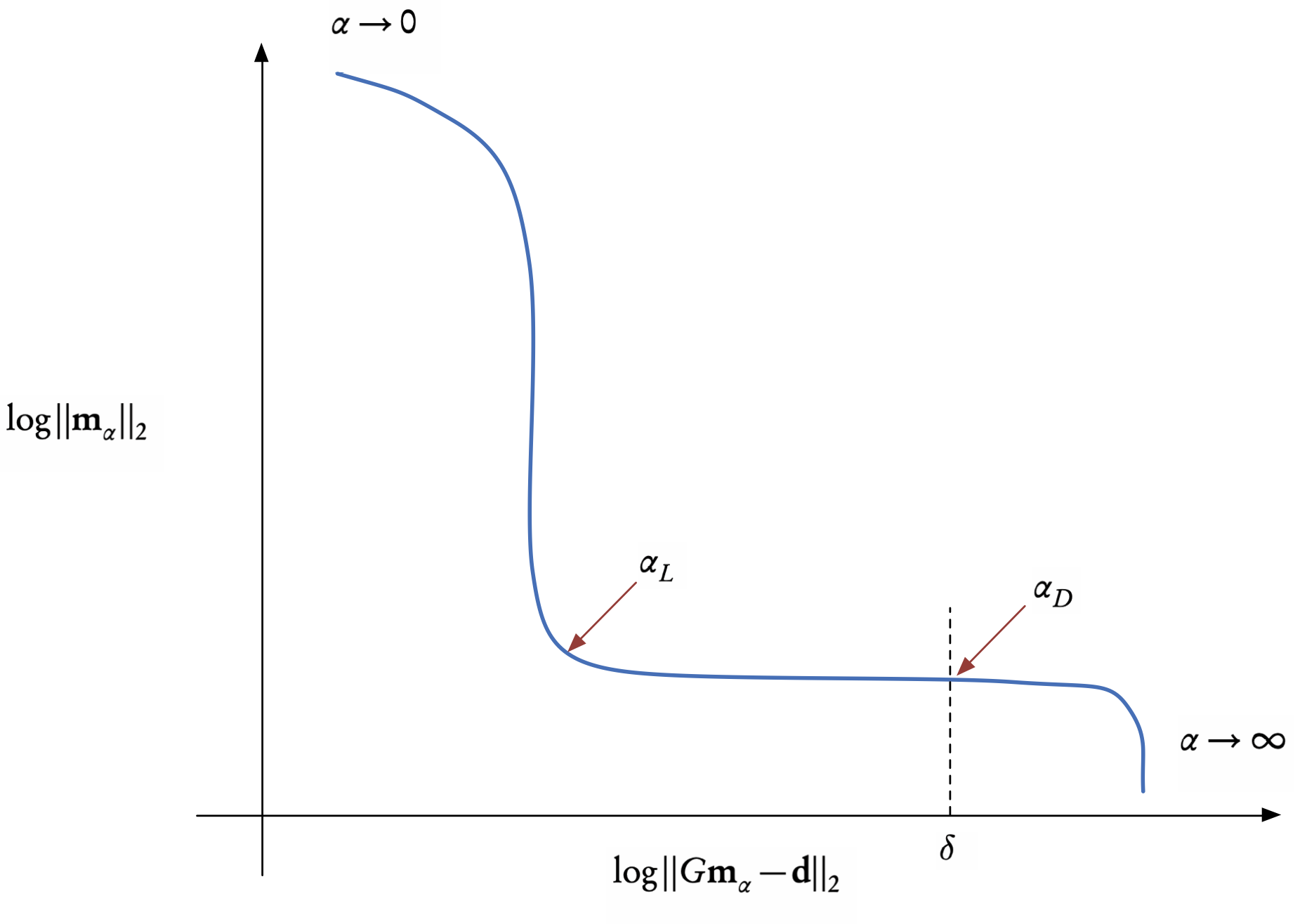
The L-curve criterion is an empirical method for picking a value of \(\alpha.\)
since \(e_{m}(\alpha)=\Vert\mathbf{m}\Vert_{2}\) is a strictly decreasing function of \(\alpha\) and \(e_{d}(\alpha)=\Vert G\mathbf{m}-\mathbf{d}\Vert_{2}\) is a strictly increasing one,
we plot \(\log e_{m}\) against \(\log e_{d}\) we will always obtain an L-shaped curve that has an “elbow” at the optimal value of \(\alpha=\alpha_{L},\) or at least at a good approximation of this optimal value see Figure 1.
This trade-off curve gives us a visual recipe for choosing the regularization parameter, reminiscent of the bias-variance trade off
The range of values of \(\alpha\) for which one should plot the curve has to be determined by either trial-and-error, previous experience, or a balancing of the two terms in the TR functional.
The discrepancy principle
choose the value of \(\alpha=\alpha_{D}\) such that the residual error (first term) is equal to an a priori bound, \(\delta,\) that we would like to attain.
on the L-curve, this corresponds to the intersection with the vertical line at this bound, as shown in Figure 1.
a good approximation for the bound is to put \(\delta=\sigma\sqrt{n},\) where \(\sigma^{2}\) is the variance and \(n\) the number of observations.1 This can be thought of as the noise level of the data.
- the discrepancy principle is also related to regularization by the truncated singular value decomposition (TSVD), in which case the truncation level implicitly defines the regularization parameter.
Cross-validation, as we explained in Chapter 9, is a way of using the observations themselves to estimate a parameter.
We then employ the classical approach of either LOOCV or \(k\)-fold cross validation, and choose the value of \(\alpha\) that minimizes the RSS (Residual Sum of Squares) of the test sets.
In order to reduce the computational cost, a generalized cross validation (GCV) method can be used.
DATA ASSIMILATION1
Definitions and notation
Analysis is the process of approximating the true state of a physical system at a given time
Analysis is based on:
observational data,
a model of the physical system,
background information on initial and boundary conditions.
An analysis that combines time-distributed observations and a dynamic model is called data assimilation.
Standard notation
A discrete model for the evolution of a physical (atmospheric, oceanic, etc.) system from time \(t_{k}\) to time \(t_{k+1}\) is described by a dynamic, state equation
\[\mathbf{x}^{f}(t_{k+1})=M_{k+1}\left[\mathbf{x}^{f}(t_{k})\right], \tag{3}\]
\(\mathbf{x}\) is the model’s state vector of dimension \(n,\)
\(M\) is the corresponding dynamics operator (finite difference or finite element discretization), which can be time dependent.
The error covariance matrix associated with \(\mathbf{x}\) is given by \(\mathbf{P}\) since the true state will differ from the simulated state (Equation 3) by random or systematic errors.
Observations, or measurements, at time \(t_{k}\) are defined by
\[\mathbf{y}_{k}^{\mathrm{o}}=H_{k}\left[\mathbf{x}^{t}(t_{k})\right]+\varepsilon_{k}^{\mathrm{o}},\]
\(H\) is an observation operator that can be time dependent
\(\varepsilon_k^{\mathrm{o}}\) is a white noise process zero mean and covariance matrix \(\mathbf{R}\) (instrument errors and representation errors due to the discretization)
observation vector \(\mathbf{y}_{k}^{\mathrm{o}}=\mathbf{y}^{\mathrm{o}}(t_{k})\) has dimension \(p_{k}\) (usually \(p_{k}\ll n.\) )
Subscripts are used to denote the discrete time index, the corresponding spatial indices or the vector with respect to which an error covariance matrix is defined.
Superscripts refer to the nature of the vectors/matrices
“a” for analysis, “b” for background (or ‘initial/first guess’),
“f” for forecast, “o” for observation, and
“t” for the (unknown) true state.
An analysis that combines time-distributed observations and a dynamic model is called data assimilation.
Standard notation—continuous system
Now let us introduce the continuous system. In fact, continuous time simplifies both the notation and the theoretical analysis of the problem. For a finite-dimensional system of ordinary differential equations, the sate and observation equations become \[\dot{\mathbf{x}}^{\mathrm{f}}=\mathcal{M}(\mathbf{x}^{\mathrm{f}},t)%\mathbf{\dot{\xf}}=\mathcal{M}(\xf,t)\] and \[\mathbf{y}^{\mathrm{o}}(t)=\mathcal{H}(\mathbf{x}^{\mathrm{t}},t)+\boldsymbol{\epsilon},\] where \(\dot{\left(\,\right)}=\mathrm{d}/\mathrm{d}t,\) \(\mathcal{M}\) and \(\mathcal{H}\) are nonlinear operators in continuous time for the model and the observation respectively.
This implies that \(\mathbf{x},\) \(\mathbf{y},\) and \(\boldsymbol{\epsilon}\) are also continuous-in-time functions.
- For PDEs, where there is in addition a dependence on space, attention must be paid to the function spaces, especially when performing variational analysis.
- With a PDE model, the field (state) variable is commonly denoted by \(\boldsymbol{u}(\mathbf{x},t),\) where \(\mathbf{x}\) represents the space variables (no longer the state variable as above!), and the model dynamics is now a nonlinear partial differential operator, \[\mathcal{M}=\mathcal{M}\left[\partial_{\mathbf{x}}^{\alpha},\boldsymbol{u}(\mathbf{x},t),\mathbf{x},t\right]\] with \(\partial_{\mathbf{x}}^{\alpha}\) denoting the partial derivatives with respect to the space variables of order up to \(\left|\alpha\right|\le m\) where \(m\) is usually equal to two and in general varies between one and four.
CONCLUSIONS
Data assimilation requires not only the observations and a background, but also knowledge of:
The challenge of data assimilation is in combining our stochastic knowledge with our physical knowledge.
Open-source software
Various open-source repositories and codes are available for both academic and operational data assimilation.
DARC: https://research.reading.ac.uk/met-darc/ from Reading, UK.
DAPPER: https://github.com/nansencenter/DAPPER from Nansen, Norway.
DART: https://dart.ucar.edu/ from NCAR, US, specialized in ensemble DA.
OpenDA: https://www.openda.org/.
Verdandi: http://verdandi.sourceforge.net/ from INRIA, France.
PyDA: https://github.com/Shady-Ahmed/PyDA, a Python implementation for academic use.
Filterpy: https://github.com/rlabbe/filterpy, dedicated to KF variants.
EnKF; https://enkf.nersc.no/, the original Ensemble KF from Geir Evensen.
References
K. Law, A. Stuart, K. Zygalakis. Data Assimilation. A Mathematical Introduction. Springer, 2015.
G. Evensen. Data assimilation, The Ensemble Kalman Filter, 2nd ed., Springer, 2009.
A. Tarantola. Inverse problem theory and methods for model parameter estimation. SIAM. 2005.
O. Talagrand. Assimilation of observations, an introduction. J. Meteorological Soc. Japan, 75, 191, 1997.
F.X. Le Dimet, O. Talagrand. Variational algorithms for analysis and assimilation of meteorological observations: theoretical aspects. Tellus, 38(2), 97, 1986.
J.-L. Lions. Exact controllability, stabilization and perturbations for distributed systems. SIAM Rev., 30(1):1, 1988.
J. Nocedal, S.J. Wright. Numerical Optimization. Springer, 2006.
F. Tröltzsch. Optimal Control of Partial Differential Equations. AMS, 2010.